
Grey Wolf Optimizer — How It Can Be Used with Computer Vision
As a bonus, get the code to apply feature extraction anywhere
This is the last part of my series of nature-inspired articles. Earlier, I had talked about algorithms inspired by genetics, swarm, bees, and ants. Today, I will talk about wolves.
When a journal paper has a citation count spanning 5 figures, you know there’s some serious business going on. Grey Wolf Optimizer [1] (GWO) is one such example.
Overview and Motivation
Like Particle Swarm Optimization (PSO), Artificial Bee Colony (ABC), and Ant Colony Optimization (ACO), GWO is also a meta-heuristic. Although there’s no mathematical guarantees to the solution, it works well in practice and does not require any analytical knowledge of the underlying problem. This allows us to query from a ‘blackbox’, and simply make use to the observed results to refine our solution.
As mentioned in my ACO article, all these ultimately relate back to the fundamental concept of explore-exploit trade-off. Why, then, are there so many different meta-heuristics?
Firstly, it is because researchers have to publish papers. A good part of their job entails exploring things from different angles and sharing the ways in which their findings bring about benefits over existing approaches. (Or as some would say, publishing papers to justify their salaries and seek promotions. But let’s not get there.)
Secondly, it is due to the ‘No Free Lunch’ theorem [2] which the authors of GWO themselves talked about. While that theorem was specifically saying there’s no free lunch for optimization algorithms, I think it is fair to say that the same is true for Data Science in general. There is no single ultimate one-size-fits-all solution, and we often have to try different approaches to see what works.
Therefore, let’s proceed to add yet another meta-heuristic to our toolbox. Because it never hurts to have another tool which might come in handy one day.
Use Case
First, let’s consider a simple classification problem on images. A clever approach is to use pre-trained deep neural networks as feature extractors, to convert each image into a feature vector.
As I had explained here, features are the strength/presence or absence of features in an image. Instead of saying a picture is worth a thousand words, it is actually more accurate to say that a picture is worth a thousand features. Really. (Or maybe 512 features, or 2048 features).
We can then apply any classical ML techniques, say for example bagging and boosting ensembles / KNN / SVM, to perform a classification. Of course, we could also use fully connected layers. The training time would be reduced significantly, and the extent of time savings exceeds just freezing the weights, because we avoid the repeated computations which would otherwise have been required for feature extraction. In addition, the feature vector can be concatenated with other information (eg. from other feature engineering techniques and/or metainformation of the image if applicable).
sklearn has an arsenal of easy-to-use APIs, and just the ensembles section alone would leave you spoilt for choices. However, it is not merely about selecting which algorithm to use; you need to select the appropriate hyperparameters as well, and there is no one-size-fits-all combination to use.
This is where GWO can be useful. We can use this metaheurestic optimization technique to select the hyperparameters instead of using a gridsearch or random search.
Before diving into the implementation details of GWO, here’s the code for features extraction.
class DataManager:
    def __init__(self, root):
        self.C, self.H, self.W = 3, 32, 32
        mean = [0.485, 0.456, 0.406]
        std = [0.229, 0.224, 0.225]
        self.transform = transforms.Compose([
            transforms.Resize(512),
            transforms.Pad((0, 0, 512, 512), fill=0, padding_mode='constant'),
            transforms.CenterCrop((512, 512)),
            transforms.ToTensor(),
            transforms.Normalize(mean, std)
        ])
        self.trainset = torchvision.datasets.Food101(
            root='food101', split='train',
            download=True, transform=self.transform
        )
        self.testset = torchvision.datasets.Food101(
            root='food101', split='test',
            download=True, transform=self.transform
        )
        self.classes = list(self.testset.class_to_idx.keys())
        self.get_loader()

    def get_loader(self):
        self.batch_size = 8
        self.trainloader = torch.utils.data.DataLoader(
            self.trainset, batch_size=self.batch_size,
            shuffle=True, num_workers=0
        )
        self.testloader = torch.utils.data.DataLoader(
            self.testset, batch_size=self.batch_size,
            shuffle=False, num_workers=0
        )

class FeatureExtractor:
    def __init__(self, dataMananger, feature_layer):
        self.dataMananger = dataMananger
        self.trainloader = self.dataMananger.trainloader
        self.testloader = self.dataMananger.testloader
        self.classes = self.dataMananger.classes
        self.artifacts_dir = "./artifact/"
        if not os.path.exists(self.artifacts_dir):
            os.makedirs(self.artifacts_dir)

        self.device = torch.device(
            torch.cuda.current_device() if torch.cuda.is_available() else 'cpu'
        )
        self.model = vgg19(weights=VGG19_Weights.DEFAULT)
        self.model.to(self.device)
        self.feature_layer = feature_layer
        self.features = []
        self.hook = self.model._modules.get(feature_layer).register_forward_hook(self.hook_fn)

    def hook_fn(self, _module, _in, _out):
        self.features.append(_out.cpu().data.numpy())

    def extract(self, loader=None):
        self.model.eval()
        features = []
        labels = []
        loader = loader or self.trainloader

        with torch.no_grad():
            for data in tqdm(loader):
                images, y_true = data
                images, y_true = images.to(self.device), y_true.to(self.device)
                output = self.model(images)
                features.extend(output.cpu().numpy())
                labels.extend(y_true.numpy())

        return features, labels
With this, you can obtain the extracted features from, say, Food101, in just three lines. The dataset is available on paperswithcode [3], which (as of 23 Fb 2024) states that “All content on this website is openly licenced under CC-BY-SA”. The definition of CC BY-SA and other types of licenses can be found here.
(Note that Food101 comprises 101,000 images, and it may take around an hour to download. It can be downloaded conveniently via torchvision or tensorflow. If you want to replicate the results below, it suffice to download just the test set. If you choose to do so, remember to comment out all the lines that call the trainset.)
dataset = DataManager('food101')
extractor = FeatureExtractor(dataset, feature_layer='avgpool')
features, labels = extractor.extract(dataset.testloader)
Note that you can use model._modules to determine the name of the relevant layer to extract. In addition, you can modify DataManager to deal with your own local dataset. To speed things up for the purpose of replication, you can add if np.random.rand() < 0.90: continue within the FeatureExtractor.extract() method() to randomly select 10% of the data. Alternatively, you can slice just the first of the unshuffled dataset, as will be the case for this demonstration.
Formulation (Math & Code)
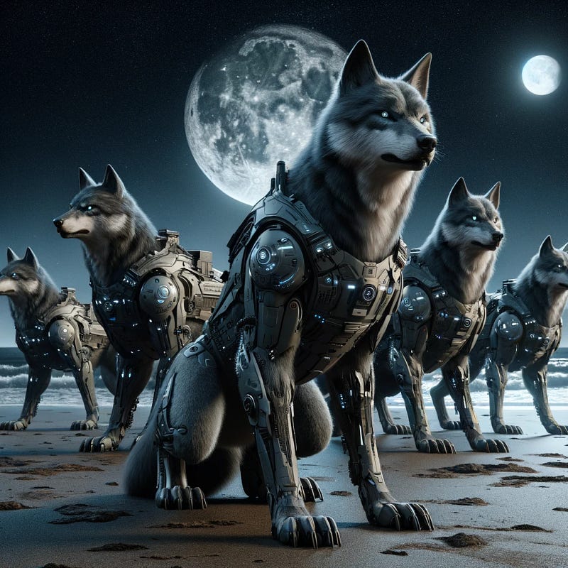
Just as I showed how ABC and ACO can be understood and utilized without knowing about a bee’s waggle dance or how ants respond to pheromones, we will learn about GWO without caring about how wolves hunt in reality.
It suffices to recognize that the alpha, beta, and delta wolves are leaders, while the omega wolves are followers, and that the behavior of followers is guided by that of their leaders.
In GWO, we have a population of ‘wolves’ that denote potential solutions, each defined by their respective fitness (which is specific to the optimization problem that you are trying to solve). The solution with the highest fitness is the alpha (α), while the second and third best solutions are the beta (β) and delta (δ), respectively.
Each solution is a point in the solution space and has n-dimensions, as explained in earlier articles. I will maintain consistency with the founding authors of GWO [1], and denote each candidate solution as X (in bold as it is a vector and not scalar). It is a function of time (strictly speaking, of iteration), and following the founding authors, the individual candidates are not denoted by any subscripts or superscripts.
The positions of the alpha, beta, and delta are denoted X_{α}, X_{β} and X_{δ}, respectively. Each wolf (ie. candidate solution) is updated every iteration via the following:

where D_{α} can be thought of as a sort of distance with respect to the alpha, although it is adjusted by a factor C₁ to encourage exploration. The resulting positions of that wolf will be the arithmetic mean of X₁, X₂ and X₃, in which equal importance has been given to the alpha, beta and delta. (Since this is a metaheuristic, you can of course use a weighted average if you prefer).
Note that ∘ is the Hadamard product, ie. element-wise multiplication between two vectors. A and C are coefficient vectors, where r₁ and r₂ are random vectors in [0,1] and components of a are linearly decreased from 2 to 0 over the iterations.

That’s as much math as you need. Seriously. It does not mean that an academic paper with over 10,000 citations must have highly complicated mathematics. As long as it works, the simpler the better.
In Python code, we can write the GreyWolfOptimizer class as follows.
class GreyWolfOptimizer:
    def __init__(self, dim, n_wolves, n_iterations):
        self.dim = dim
        self.n_wolves = n_wolves
        self.n_iterations = n_iterations
        self.alpha_wolf = None
        self.beta_wolf = None
        self.delta_wolf = None


    def optimize(self, features, labels, upper_bound, lower_bound):
        #wolves = np.random.rand(self.n_wolves, self.dim)
        wolves = lower_bound + (upper_bound - lower_bound) * np.random.rand(self.n_wolves, self.dim)
        fitness = np.zeros(self.n_wolves)

        self.X_train, self.X_val, self.y_train, self.y_val = train_test_split(features, labels.ravel(), test_size=0.2)

        for iteration in tqdm(range(self.n_iterations)):
            for i in range(self.n_wolves):
                fitness[i] = self.fitness_function(wolves[i])
            print("fitness: ", fitness)

            sorted_indices = np.argsort(fitness)
            delta_id, beta_id, alpha_id = sorted_indices[-3:]
            self.alpha_wolf = wolves[alpha_id]
            self.beta_wolf = wolves[beta_id]
            self.delta_wolf = wolves[delta_id]

            for i in range(self.n_wolves):
                A1 = 2*np.random.uniform(high=1 - iteration/self.n_iterations)
                A2 = 2*np.random.uniform(high=1 - iteration/self.n_iterations)
                A3 = 2*np.random.uniform(high=1 - iteration/self.n_iterations)  # simplified to be linearly decreasing with iteration
                C1, C2, C3 = 2 * np.random.rand(), 2 * np.random.rand(), 2 * np.random.rand()
                D_alpha = abs(C1 * self.alpha_wolf - wolves[i])
                D_beta = abs(C2 * self.beta_wolf - wolves[i])
                D_delta = abs(C3 * self.delta_wolf - wolves[i])
                X1 = self.alpha_wolf - A1 * D_alpha
                X2 = self.beta_wolf - A2 * D_beta
                X3 = self.delta_wolf - A3 * D_delta
                wolves[i] = np.clip((X1+X2+X3) / 3, lower_bound, upper_bound)

        return self.alpha_wolf


    def fitness_function(self, hyperparams):
        n_estimators = int(hyperparams[0]*50 + 60)            # 10 to 110
        max_depth = int(hyperparams[1]*8 + 12)                # 4 to 20
        min_samples_split = int(np.exp(hyperparams[2]*2 + 3)) # 2 to 148
        max_features = int(hyperparams[3]*50 + 60)            # 10 to 110

        clf = RandomForestClassifier(
            n_estimators=n_estimators, max_depth=max_depth, min_samples_split=min_samples_split, max_features=max_features
        )
        clf.fit(self.X_train, self.y_train)
        y_pred = clf.predict(self.X_val)
        accuracy = accuracy_score(self.y_val, y_pred)
        return accuracy    # to maximize
With this, we can determine the hyperparameters to be used for building an ML model to predict train_labels from train_features, both obtained from the FeatureExtractor class.
lower_bound, upper_bound = np.array([-1, -1, -1, -1]), np.array([1, 1, 1, 1])
dim = len(upper_bound)

n_wolves = 10
n_iterations = 5
optimizer = GreyWolfOptimizer(dim, n_wolves, n_iterations)
optimal_hyperparams = optimizer.optimize(features, labels, upper_bound, lower_bound)
Results
Note that the point of this article is not to show some record-breaking model performance. Such demonstrations would not be reproducible by the vast majority of readers, as that would require lengthy training. I do not believe in such ‘take-my-word-for-it’ stuff; you should always attempt to replicate the results on your own computer.
Instead, the focus here is to teach you the approach of utilizing GWO to select hyperparameters of a classification model. This could be applied to feature vectors extracted from some pre-trained network, or simply to tabular data. By following the steps above, you can easily reproduce the results in a matter of minutes.
The feature extraction takes around 1 second per image (each 512-by-512 pixels). For 10% of Food101 test set, the 2500 images adds up to tens of minutes (just go do other stuff and come back later). Good thing this feature extraction process only happens once, and thereafter, each image can be represented much more concisely with its feature vector.

To establish a baseline, we use the default hyperparameters; the model as well as evaluation metrics are obtained in a couple of seconds. On the approximately 1000 unseen samples, this method gives an accuracy of 57% and F1 score of 56–57%.
clf = RandomForestClassifier()
clf.fit(optimizer.X_train, optimizer.y_train)
y_pred = clf.predict(optimizer.X_val)
print(classification_report(optimizer.y_val, y_pred))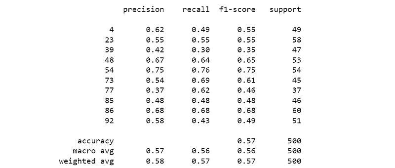
Now, we perform the GWO and use the suggested hyperparameters as follows. This gives a two percentage points improvement in accuracy as well as F1 score after a short 5-minute search with 5 iterations.
n_estimators = int(optimal_hyperparams[0]*50 + 60)
max_depth = int(optimal_hyperparams[1]*8 + 12)
min_samples_split = int(np.exp(optimal_hyperparams[2]*2 + 3))
max_features = int(optimal_hyperparams[0]*50 + 60)
clf = RandomForestClassifier()
clf.fit(optimizer.X_train, optimizer.y_train)
y_pred = clf.predict(optimizer.X_val)
print(classification_report(optimizer.y_val, y_pred))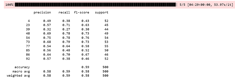
Notice that the search space is kept to [-1, 1], and I use things like np.exp(optimal_hyperparams[j]). This ensures that the different dimensions of the search space are comparable to one another. In addition, it allows us to search logarithmically, which is especially important for things like learning rates.
Keep in mind that GWO is just one of many optimization techniques, and that there is no single best approach as supported by the ‘No Free Lunch’ theorem. Also, hyperparameter tuning is one use-case of GWO, but certainly not the only.
Conclusion
In this article, I explained the mathematics associated with Grey Wolf Optimizer, along with the code required to implement it. I applied this to a simple use case of tuning the hyperparameters of a random forest classifier. In addition, I also gave the code for efficiently extracting features from pretrained deep neural networks, with which you can apply an assortment of other ML techniques and show value-add as a data scientist.
Though not demonstrated here, the founding authors of GWO [2] wrote that this algorithm outperforms PSO and GSA (Gravitational Search Algorithm) for the majority of multimodal functions tested.
Future
While there exists other nature inspired algorithms, such as those inspired by firefly and cuckoo, I will not continue with those. And hence, this article is the last of its series.
Moving forward, I plan to write about things related to computer vision, which is the domain which really got me started as a data scientist, and what I spent the initial years of my career on. I also intend to write about how we can use AWS to showcase our work and stand out in job interviews.
References
[1] S. Mirjalili, S. M. Mirjalili, and A. Lewis, Grey wolf optimizer (2014), Advances in engineering software, 69:46–61.
[2] D. H. Wolpert and W. G. Macready, No free lunch theorems for optimization (1997), IEEE transactions on evolutionary computation, 1(1): 67–82.
[3] L. Bossard, M. Guillaumin, and L. Van Gool, Food-101 (2014), Papers With Code. Retrieved from https://paperswithcode.com/dataset/food-101.


