
Ant Colony Optimization — Intuition, Code & Visualization
Where it stands out from other swarm algorithms
This article is a continuation of my nature-inspired series.
Previously, I talked about Evolutionary Algorithm (EA), Particle Swarm Optimization (PSO), as well as Artificial Bee Colony (ABC). Nature is everywhere, and there’s certainly more areas where humans can benefit by learning from nature.
Today, we focus on ants.
As children, we learnt that ants are hardworking and cooperative. What our parents hadn’t taught us was that ants collectively form a highly sophisticated swarm that communicates with one another effectively.
Knowledge of ants or pheromones (or any diffusion of any chemicals) is not required here at all. These are just names used for the purpose of packaging. I’ve shown previously that you do not need the slightest knowledge of a bee’s waggle dance in order to appreciate or utilize ABC, nor do you need to learn about genes or mutations or reproduction to apply EA.
All you need is an understanding of English to have the intuition, along with very basic math and python programming skills. While I will be showing some mathematics for completeness, which includes Greek symbols, it is really just for the purpose of completeness. It would be a great pity if these technical-sounding words or symbols stop you from learning these great algorithms, so do yourself a favor and read on.
Use Case
Before going into any math or code, or even how the algorithm works at a high level, it makes sense to see the relevance. After all, if it doesn’t help to solve a problem, why bother in the first place?
The classic example which lecturers or proponents of Ant Colony Optimization (ACO) use is the double bridge experiment [1], which shows that this algorithm can be used to find the shortest path between two points.
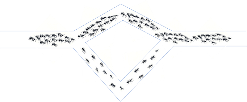
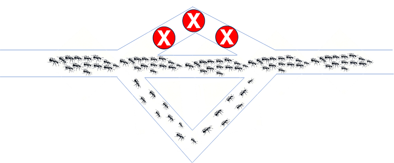
Moreover, it is robust to changes in the environment. If existing paths get obstructed, and/or if new paths arise, the solution can be updated with ease, instead of re-computing everything from scratch.
You’ll find lots of resources on the above example, so let’s do something more fun over here. Let’s consider the Travelling Salesman problem, which is effectively a combinatorics problem that can be solved using, say, Evolutionary Algorithm (code and visualization of solution process here).
The issue is, what happens when the graph (ie. cities on the map) changes, and nodes get added or removed? At the end of this article, you will be equipped with the knowledge to solve such problems effectively.
Variants of ACO
There are different variants of ACO. For the purpose of keeping this article accessible to everyone, I will just discuss the Simple ACO [2], which would serve as the foundation should you choose to delve further into the improved variants such as Ant System [3], Ant Colony System [4], and MAX-MIN Ant System [5].
P.S. The word ‘simple’ is not given by me; it is by the author who has the many papers on ACO.
Formulation (Math)
ACO is ideal for finding the shortest path on a graph. Given a set of nodes and edges, the probability of an ant k, which is currently in node i, to the next node j, is proportional to the pheromone τᵢⱼ on the edge of nodes i and j, normalized with respect to sum of pheromone on all possible candidate edges. Nᵢᵏ refers to the eligible nodes which ant k can visit from node i.

Edges leading to the ineligible nodes (eg. cities which had already been visited) are automatically excluded here, such that the probability of reaching those nodes is 0. The pheromone on those edges has no influence towards the computation of probabilities among the valid nodes.
Consequently, all ants will eventually reach a destination node (even though it may have taken a highly ineffective route to get there). Next, the ants return to its source (just like in real life) and along the way, pheromone is added to the edge traversed.

In the equation above, ant k adds ∆τᵏ worth of pheromone to the edge ij. The total pheromone along that edge is τᵢⱼ, which is a function of time t. All things being equal, this means that the probability pᵢⱼ of that edge being visited will be increased (though the effect could be outweighed by the increase in pheromone along other edges if the denominator Στᵢⱼ increases by a greater proportion).
The pheromone ∆τᵏ added by ant k is simply 1/Lᵏ, where Lᵏ is the length of its path. Shorter paths are more favorable, and hence a greater quantity will be added to those edges traversed by that ant.
To avoid quickly converging to a sub-optimal solution, as well as avoid excessive dependence on the initialization values, the pheromone on each edge will be decayed exponentially.

Simple Example
As an illustration, consider ACO with just one single ant, which starts at node 1, with pheromone as indicated next to each edge. For clarity, only τ₁₂, τ₁₃, τ₁₄, and τ₁₅ are shown.
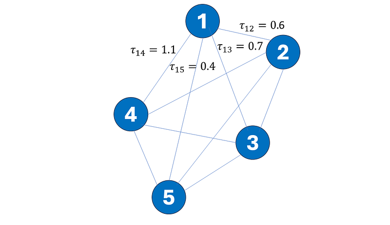
Similar to how selections in EA are performed, there are actually different ways to select an edge from the given τᵢⱼ. Ultimately, it all comes down to the fundamental concept of the explore-exploit trade-off, which itself forms the bedrock of Reinforcement Learning.
For simplicity, we can use the straightforward roulette selection approach. Note that the superscript k is omitted here since we are considering just a single ant. Where there are different ants, the denominator may differ according to each ant’s path history, such that the valid candidate nodes Nᵢᵏ may differ for ants in any particular node.

Suppose the ant travels from node 1 to node 2. N₂ᵏ will thereafter comprise only nodes 3, 4 and 5. Let’s consider the scenario where our single ant traversed the path [1–2–4–3–5–1]. Hypothetical values for Lᵢⱼ and τᵢⱼ are given in the illustration below.
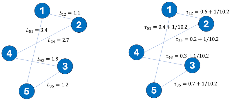
Each edge that had been traversed will have 1/10.2 of pheromone added, where the denominator had been computed from L₁₂+L₂₄+L₄₃+L₃₅+L₅₁. We assume that Lᵢⱼ and Lⱼᵢ are equal, i.e. the cost of travelling from nodes i to j (or city i to j) is the same as from nodes j to i. Consequently, directionality can be ignored when considering the pheromone between two nodes, ie. τᵢⱼ equals τⱼᵢ. After adding pheromone to edges that had been visited, the evaporation process will be invoked, where τ will be decayed by a constant factor.
Based on the new updated values of τᵢⱼ, the simulation process is repeated, and new paths will be traversed following the updated probabilities.
Formulation (Code)
The following python code can be used to implement ACO according to the approach discussed above.
import numpy as np
import random
from tqdm import tqdm
from copy import deepcopy
import matplotlib.pyplot as plt

class SimpleACO:
    def __init__(self, salesman, n_ants, rho):
        self.salesman = salesman
        self.n_ants = n_ants
        self.rho = rho
        self.pheromone = 0.01*np.ones((self.salesman.num_cities, self.salesman.num_cities))

    def update_map(self, new_salesman):
        num_old_cities = len(self.pheromone)
        retain = deepcopy(self.pheromone)
        self.salesman = new_salesman
        self.pheromone = 0.01*np.ones((self.salesman.num_cities, self.salesman.num_cities))
        self.pheromone[:num_old_cities,:num_old_cities] = retain

    def run(self, n_iterations):
        best_distance = float('inf')
        best_solution = None

        for _ in tqdm(range(n_iterations)):
            solutions = [self.generate_path() for _ in range(self.n_ants)]
            self.update_pheromone(solutions)

            for solution in solutions:
                distance = -self.salesman.fitness(solution)
                if distance < best_distance:
                    best_distance = distance
                    best_solution = solution

        return best_solution

    def generate_path(self):
        path = [random.randint(0, self.salesman.num_cities - 1)]
        while len(path) < self.salesman.num_cities:
            next_city = self.choose_next_city(path[-1], path)
            path.append(next_city)
        path.append(path[0])
        return path

    def update_pheromone(self, solutions):
        self.pheromone *= (1 - self.rho)
        for solution in solutions:
            for i in range(len(solution) - 1):
                self.pheromone[solution[i]][solution[i+1]] += 1 / -self.salesman.fitness(solution)

    def choose_next_city(self, current_city, path):
        probabilities = []
        for city in range(self.salesman.num_cities):
            if city not in path:
                probabilities.append(self.pheromone[current_city][city])
            else:
                probabilities.append(0)

        probabilities = np.array(probabilities)/np.sum(probabilities)
        next_city = np.random.choice(range(self.salesman.num_cities), p=probabilities)
        return next_city
Note that the initialized values in self.pheromone has to be commensurate with the typical amount of pheromone added in each iteration. If it is much larger, the ‘explore’ component of the solution would dominate the ‘exploit’ component.
In a previous article on Evolutionary Algorithm, I had already written a class for TSP. For your convenience, I am appending it here.
class Salesman:
    def __init__(self, num_cities, x_lim, y_lim, read_from_txt=None):
        if read_from_txt:
            self.city_locations = []
            f = open(read_from_txt)
            for i, line in enumerate(f.readlines()):
                if i==num_cities:
                    break
                node_val = line.split()
                self.city_locations.append(
                    (float(node_val[-2]), float(node_val[-1]))
                )
            self.num_cities = len(self.city_locations)
            self.x_lim = np.max(np.array(self.city_locations)[:,0])
            self.y_lim = np.max(np.array(self.city_locations)[:,1])

        else:   # generate randomly
            self.num_cities = num_cities
            self.x_lim = x_lim
            self.y_lim = y_lim
            x_loc = np.random.uniform(0, x_lim, size=num_cities)
            y_loc = np.random.uniform(0, y_lim, size=num_cities)
            self.city_locations = [
                (x,y) for x,y in zip(x_loc,y_loc)
            ]
        self.distances = self.calculate_distances()


    def calculate_distances(self):
        distances = np.zeros((self.num_cities, self.num_cities))
        for i in range(self.num_cities):
            for j in range(i + 1, self.num_cities):
                dist = np.sqrt((self.city_locations[i][0] - self.city_locations[j][0]) ** 2 + (self.city_locations[i][1] - self.city_locations[j][1]) ** 2)
                distances[i][j] = distances[j][i] = dist
        return distances


    def fitness(self, solution):
        total_distance = 0
        for i in range(self.num_cities - 1):
            total_distance += self.distances[solution[i]][solution[i+1]]
        total_distance += self.distances[solution[-1]][solution[0]]   ###
        fitness = -total_distance
        return fitness


    def visualize(self, solution, save_id=None):
        n = len(solution)
        assert n == len(self.city_locations), 'The solution must correspond to all cities'
        for i, (x,y) in enumerate(self.city_locations):
            plt.plot(x, y, "ro")
            plt.annotate(i, (x, y))

        ordered_cities = [self.city_locations[idx] for idx in solution]
        x_coord = [x for (x,y) in  ordered_cities] + [ordered_cities[0][0]]  ###
        y_coord = [y for (x,y) in  ordered_cities] + [ordered_cities[0][1]]  ###
        distance = -self.fitness(solution)

        plt.plot(x_coord, y_coord, "gray")
        plt.title("Connected cities (%.1f) according to solution" % distance)
        if save_id is not None:
            filename = "results/plot_%03d.png" % save_id
            plt.savefig(filename, bbox_inches='tight')
            plt.close()
        else:
            plt.show()
A simple modification is made to three lines, where the lines involved have ### added. In the previous use case, I gave an example of planning a trip around Europe — in such cases we simply want to visit each city once, and not form a closed loop to end at the very first city started. (I’m pretty sure you would purchase two one-way flight tickets, and depart from a different city).
The code has been modified to form a complete loop above, hence you now have the flexibility of choosing which approach fits your use-case better.
Results
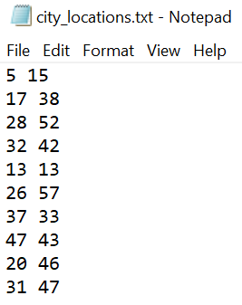
Consider 10 cities, having locations saved in and read from a txt file.
All that is left to do is to define our Salesman class and SimpleACO class, which comes with the .run() and .visualize() methods.
salesman = Salesman(num_cities=-1, x_lim=100, y_lim=100, read_from_txt='city_locations.txt')
aco = SimpleACO(salesman, n_ants=20, rho=0.1)
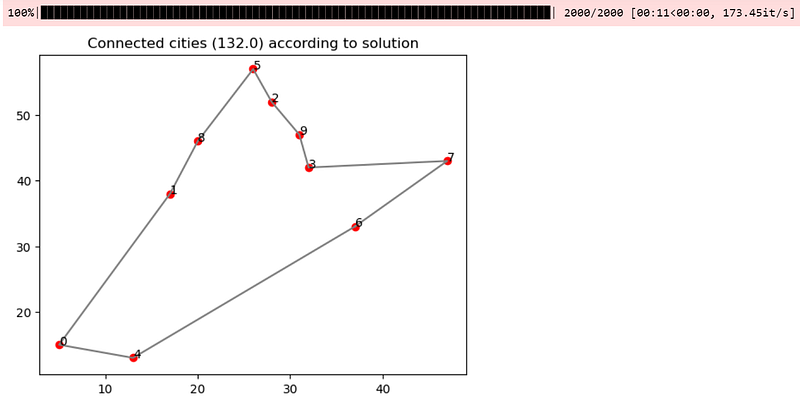
best_solution = aco.run(n_iterations=2000)
salesman.visualize(best_solution[:-1])In just a couple of seconds, the following output can be obtained.
The reason it works is because of the following intuition:
- All edges has a probability of being visited.
- When the number of ants and iterations are sufficiently large, all edges will eventually be explored.
- Edges which are part of a shorter path will have a larger amount of pheromone added to it.
- In a shorter route, it is likely that edges which form that route are more ideal than edges which form other longer routes.
- By selected edges according to the amount of pheromone, ants are inclined towards selecting ideal paths.
Note that the above results had been obtained after a couple of runs. There are some runs in which the results are bad. This is quite unlike the case for Evolutionary Algorithm, where the results are generally near optimal across different runs (to compare the results, you first need to define Evolutionary class from here).
evo = Evolutionary(salesman)
best_genome = evo.run_evolution(
    population_size=200, generation_limit=1000, crossover='pmx'
)
salesman.visualize(best_genome)
Nonetheless, this should not be a deal-breaker in learning a new algorithm. One can always perform multiple runs using different algorithms, and simply choose the best solution.
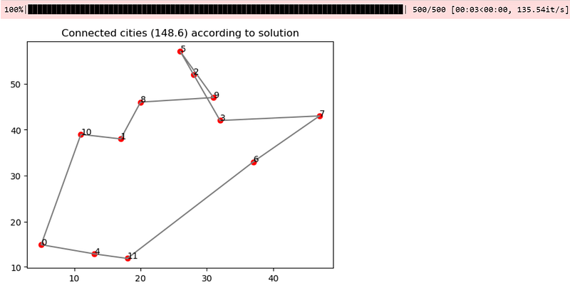
What happens if the cities change? In the case of cities being added to the list, it is straightforward to perform an incremental update using .update_map() with the new configurations, before using .run(). The benefit of doing so is that the pheromone between existing edges can be re-used.
new_salesman = Salesman(num_cities=-1, x_lim=100, y_lim=100, read_from_txt='city_locations_new.txt')
aco.update_map(new_salesman)
new_best_solution = aco.run(n_iterations=500)
new_salesman.visualize(new_best_solution[:-1])
Do keep in mind that the code above assumes that all existing cities (nodes) are unchanged, with the new ones added at the bottom of the list. If there are cities being removed, you will need to keep the correct portion of the .pheromone attribute so that the relationship between existing nodes are maintained.
Conclusion
In this article, you’ve learnt the mathematics behind the baseline implementation ACO, its associated intuition, as well as the code needed to implement this algorithm to solve the TSP. As promised, you don’t need any knowledge of ants or chemistry to tap on the benefits of this algorithm.
You’ve also seen how the codes are used in a plug-and-play manner, where the SimpleACO class (for ACO; introduced here) integrates seamlessly with the Salesman class (for TSP) that was originally written for Evolutionary class (for EA).
References
[1] M. Dorigo, M. Birattari, and T. Stutzle, Ant colony optimization (2006), IEEE computational intelligence magazine, 1(4), 28–39.
[2] M. Dorigo and T. Stützle, An experimental study of the simple ant colony optimization algorithm (2001). In 2001 WSES International Conference on Evolutionary Computation.
[3] M. Dorigo, V. Maniezzo, and A. Colorni. Ant System: Optimization by a colony of cooperating agents (1996), IEEE Transactions on Systems, Man, and Cybernetics — Part B, 26(1):29–41.
[4] M. Dorigo and L. M. Gambardella. Ant Colony System: A cooperative learning approach to the traveling salesman problem (1997), IEEE Transactions on Evolutionary Computation, 1(1):53–66, .
[5] T. Stützle and H. H. Hoos, MAX–MIN Ant System (2000), Future Generation Computer Systems, 16(8):889–914.


