Gradient Descent Intuition — How Machines Learn

The algorithm to find the “lowest-cost” state in which the ML system can exist.

Gradient descent is an algorithm to find the minimum of a function. In machine learning, the difference between the predicted and the actual value is called error. All error, across all datapoints, when added together is known as the cost.

Naturally, we would want to minimize the function that represents this cost — Cost Function. When the cost function cannot be differentiated easily Gradient Descent does the job for us.

Step by step we descend, GD is the means to our end - The AI Poet

Source: Some creative soul on Tumblr and Family Guy geniuses

Where in Machine Learning does Gradient Descent figure?

Gradient descent figures in the training phase of any machine learning algorithm. For example, neural networks are trained by using a technique called Backpropagation. Gradient descent forms a very important part of backpropagation.

Gradient descent is a very popular method to tune the parameters of a machine learning model — so as to attain the minimum error state.

A machine learning algorithm is about telling the machine to learn data’s behavior. Given that a machine can only understand 0’s and 1’s it is necessary to represent data by a mathematical model. Any mathematical model would invariably have some parameters e.g. a straight line has two parameters — slope and intercept : y = m*x+b.

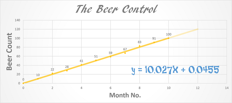
As explained in the linear regression article the intent there is to fit a straight line to our data. That essentially means tune the parameters m and b in a way that the line represents the data. (Left Figure)

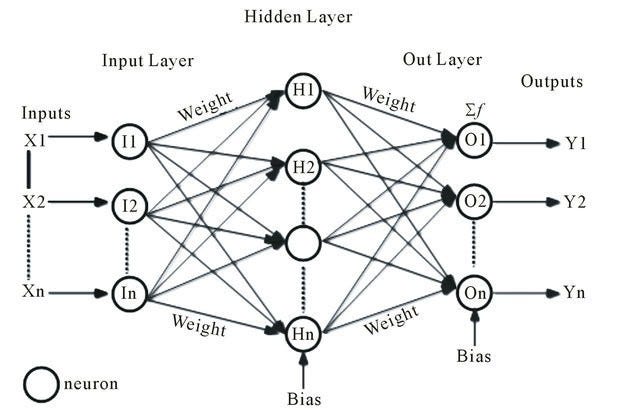
**Left** :Parameters for Straight Line Model | **Right**: Params for Neural net (Source: http://tuxar.uk/brief-introduction-artificial-neural-networks/)

Other mathematical models also contain parameters e.g. all the weights of hidden layers in neural networks are parameters for that network. The weight is the strength of connection between a neuron in one layer and another neuron in the next layer. Each of these weights becomes a parameter that needs to be tuned such that our model best represents the data and gives accurate predictions in future. (Right Figure).

This tuning of parameters is where gradient descent figures.

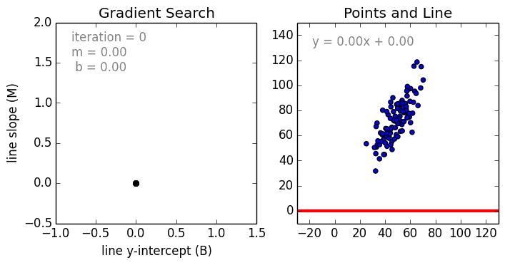
Nikhil Raghavendra describes very beautifully in his article this tuning of parameters. Notice how m and b are changing.

We keep tuning the parameters until the cost function is at its minimum.

How does Gradient Descent work?

Ok now that we know that gradient descent is used to find the minimum error (lowest cost) state for our machine learning model, let’s see how it actually works.

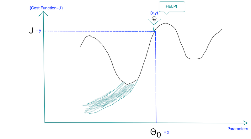
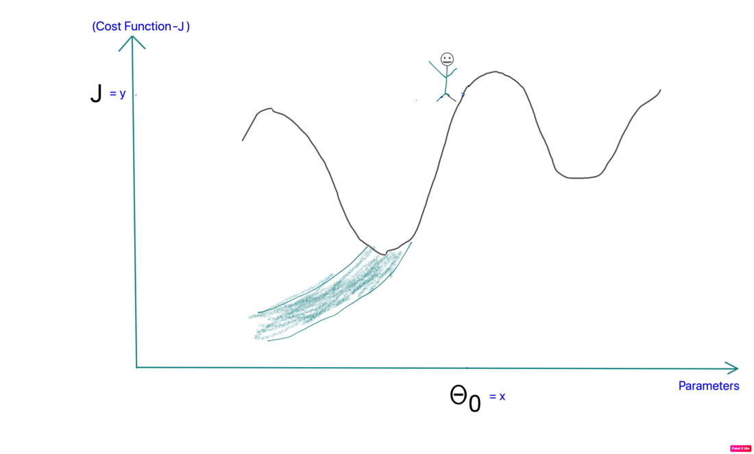
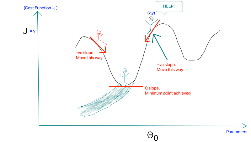
Imagine a lost hiker. He is lost somewhere near the top of the mountain and doesn’t know which way to go. He needs to find his way to the valley from where he can walk off.

That’s essentially how gradient descent also works.

Randomly choose the starting point for our hiker.
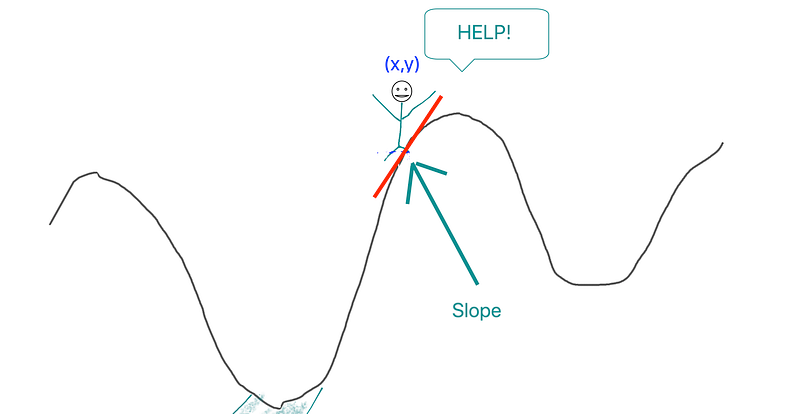
We measure the slope of the mountain at the point where he is standing
We take a step downhill
The step size is proportional to the absolute magnitude of the slope at that point. This means that the steeper the slope the bigger our step.

Now let’s try to equate this analogy to our actual problem.

The mountain = Cost Function
Hiker’s ground position = Parameters
Slope of mountain = Derivative of cost function
Step = change in parameters
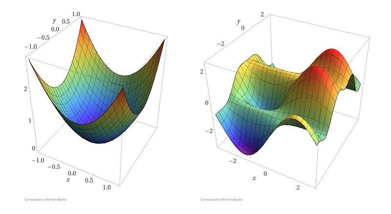
If the cost function contains only 1 parameter then we get a mountain as shown above. If the cost function contained 2 parameters the mountain would be 3-D and would look like one of these two:

Source: https://blog.paperspace.com/intro-to-optimization-in-deep-learning-gradient-descent/

Let’s get a little mathematical

To understand Gradient Descent we need to understand the following things

Parameters
Cost Function
Gradient = Derivative of Cost Function
Learning Rate
Update Rule

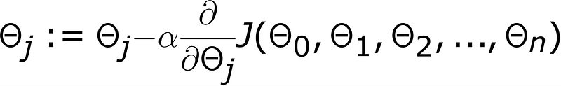
1) Parameters

Let’s say we have n+1 parameters denoted by

2) Cost Function

On these thetas depends the cost function. The cost function is basically different ways to sum up the error — the difference b/w predicted and actual. Without going into how a cost function looks like let’s just denote it by the letter J. Because J is a function of all the parameters we write it as

For 1 variable case we will just have θ₀ and J(θ₀)

3) Gradient = Slope

To compute the slope we compute the derivative of the loss function at that point. The notation below implies the partial derivative of loss function w.r.t to theta_j.

Note that this is positive slope. Had the hiker been on the left peak he would have gotten a -ve slope

4) Learning Rate

Learning rate is denoted by the character α. Alpha controls how big a step do we take during our descent. Since our step is determined by the derivative as shown above, alpha gets multiplied with this derivative to control the step size.

If alpha is too small the hiker will take too long to come to the valley i.e. the gradient descent will take too long to converge

Very small alpha leads to extremely small steps which causes slow convergence

If alpha is too big the hiker will move very fast and miss the valley and overshoot.

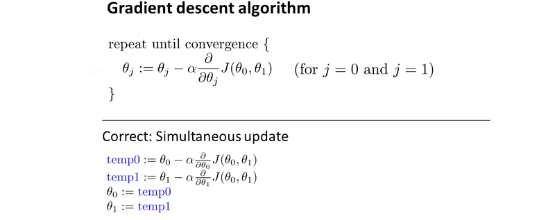
Large alpha doesn’t let the gradient descent converge

5) Update rule

Finally gradient descent is nothing but the update rule. The update rule updates all the parameters simultaneously. A parameter’s current value is subtracted by the step value. The formula for that comes from combining all the above terms.

Update rule. We do this for all **thetas** simultaneously

NOTE: If slope is negative the second term will become positive (due to the minus sign) and that will cause the parameter to increase in value. So the hiker moves a little bit to the right when the slope is -ve. If the slope is +ve theta decreases and the hiker moves a little to the left. When slope is 0 the 2nd term becomes 0 and theta doesn’t change its value.

In Summary

Take an initial guess of all thetas/parameters
Apply the update rule until the cost function reaches a stable minimum value

Summary. Source: Machine Learning Course by Andrew Ng

Things to observe

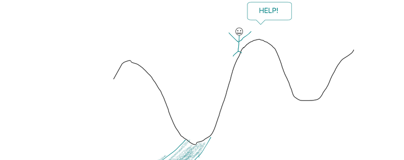
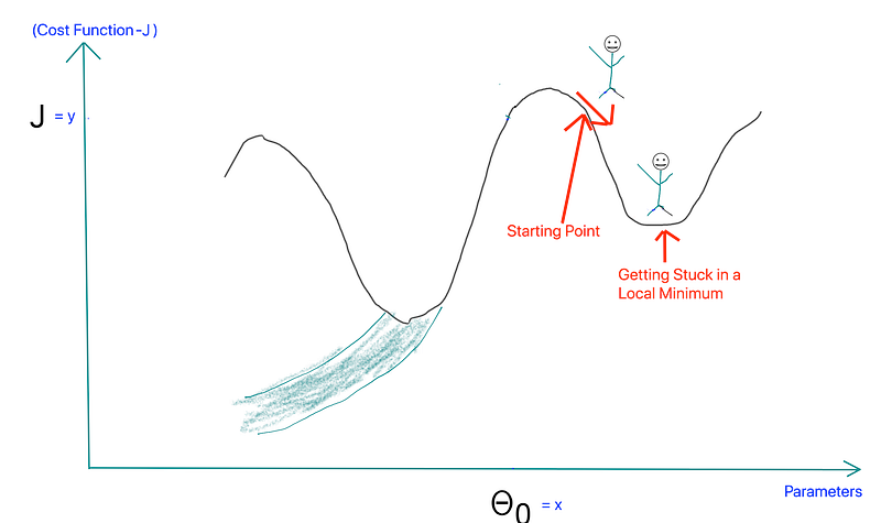
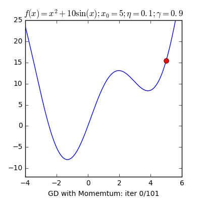
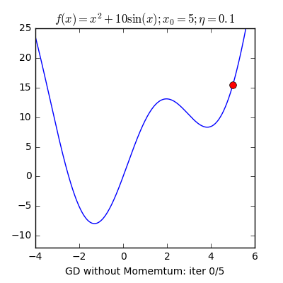
Local Minima: The 1st step of gradient descent is always random initialization. Now we may be luck and initialize our theta to be at the minimum but that is rare. What is more probable is that we might end up starting our theta at a point from where it can never reach the global minimum. It might get stuck in a local minimum. For example if the hiker were to start from the right of the peak he would get stuck in the local minimum.

Step Size: The steeper the slope bigger the steps we take. This happens because steeper slope leads to a larger derivative value and that changes theta by a bigger percentage. So higher up on the peak the hiker moves fast and as we get closer to the minimum we slow down.

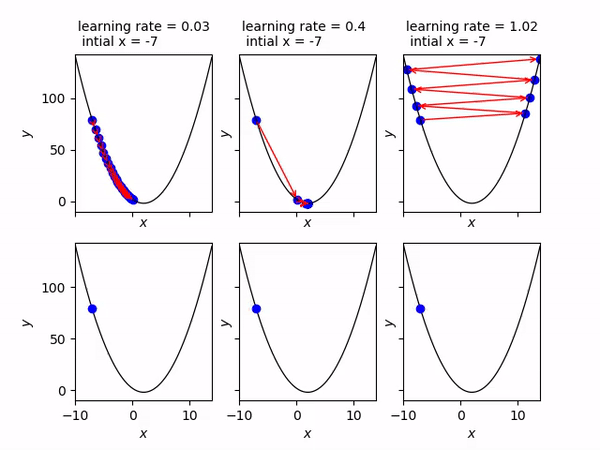
Convergence: If alpha is too small we may never converge and if it is too big we might overshoot. Below you can see that an alpha = 0.03 is too slow, alpha = 0.4 is just right and alpha = 1.02 is too big and gradient descent diverges.

Flexibility with algorithms: Since gradient descent doesn’t concern itself with the mathematical model and is only dependent on the cost function it is applicable to a wide variety of machine learning algorithms — linear regression, logistic regression, neural networks etc.
Momentum: Remember the local minimum problem? Sometimes people use the concept of momentum to prevent GD from getting stuck. The momentum term makes sure that the system stabilizes only at a global minimum.

Left: Momentum lets the system achieve global minimum. Right: Stuck in a local minimum

X8 aims to organize and build a community for AI that not only is open source but also looks at the ethical and political aspects of it. We publish an article on such simplified AI concepts every Friday. If you liked this or have some feedback or follow-up questions please comment below.

Thanks for Reading!