
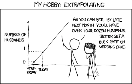
Practical aspects — Linear Regression in layman terms
I won $100 on Monday, $200 on Tuesday, $300 on Wednesday, how much would I win on Thursday? If you answered $400 you just did linear regression!
The everyday predictions we make are mostly driven by linear regression. The number of miles you’ll run based on the time you run for and the energy level you have, the number of books you’ll read based on your new year resolution and last year’s number, the bonus you’ll get based on company performance and your own, house prices based on land size etc.
We constantly make predictions, e.g. how far we can throw the ball based on how forcefully we throw, time to travel given traffic conditions etc. Linear regression can be used as the simplest tool to make predictions on such relations. Not all of the above examples follow a linear trend though. Hence it is important to understand that even the linear regression can be the first attempt at understanding the data it may not always be ideal.
But look at the pattern above! One thing is common
‘Make a Prediction’ based on ‘some information’
Terminology-wise
‘prediction’ = dependent variable and ‘some information’ = independent variables.
So we know that given independent variables we can draw conclusion about a dependent variable. The other significant feature of a simple linear regression is that it is a straight line.
Example 1 — Linear Coin
Without going into too much jargon let’s jump into examples.
Let’s assume there is a new cryptocurrency out there called LinearCoin. As opposed to the other crypto currencies, it grows stably. No surges, no dips. The CyptoPundits predict that on an average its value will grow by $10 every year.
On an average points to trend. Trend is the key here.
In 2010, it was $20. According to this prediction, in 8 years its value should increase by $10*8 = $80. It should be $100.
When plotted its real trend looks something like this. The red dots indicate the actual value each year.
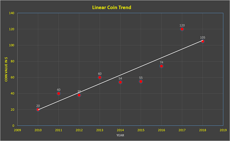
There is no year when the LinearCoin actually rises by $10 but over the course of 8 years it does grow by roughly $80. Based on the white line that Linear Regression generates you can predict what the value will be in the year 2018 or 2019 or even between the year 2012 and 2013. The prediction might not be spot on but will be close enough!
Linear Regression provides you with a straight line that lets you infer the dependent variables
The above examples is a time-series (more on time-series in a separate article) but it doesn’t mean linear regression only works on time series. In fact, linear regression rarely is useful for time series, because when applied on time series it becomes extrapolation (predicting the future), which is rarely linear.
Linear regression finds better use in examples like the amount of rainfall that affects cotton crop yield or the number of new users that sign up for Facebook vs the revenue FB generates.
Example 2 — Beer Control
The above examples conveys the basic idea but how does the math work? Linear regression at the end generates values for parameters that represent a line.
- Let’s first look at how a straight line is represent in coordinate geometry.
- This straight line needs to fit the data. Then we will look at how we can manually fit the line to the data.
- Finally we look at how machines carry out the fitting process — Linear Regression
The equation Y=mX+C
In terms of coordinate geometry if dependent variable is called Y and independent variable is called X then a straight line can be represented in terms of Y and X as Y = m*X+c. Where m and c are two numbers that linear regression tries to figure out to estimate that white line.
Look at the figure below. Let’s say you decide to become conscious of how much you drink. You count the number of beer pints that you drink. If we plot it by number of months it looks something like the graph below. Here X is the number of months and Y is the number of beers you have drunk by that month.
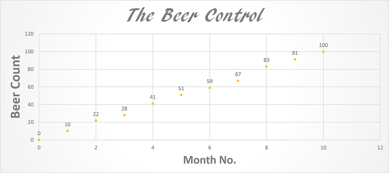
What do you see? How many beers roughly do you drink each month? A simple look shows you drink 10 pints per month (Not bad!).
What do you expect the trendline to look like? How many beers at the end of the year?
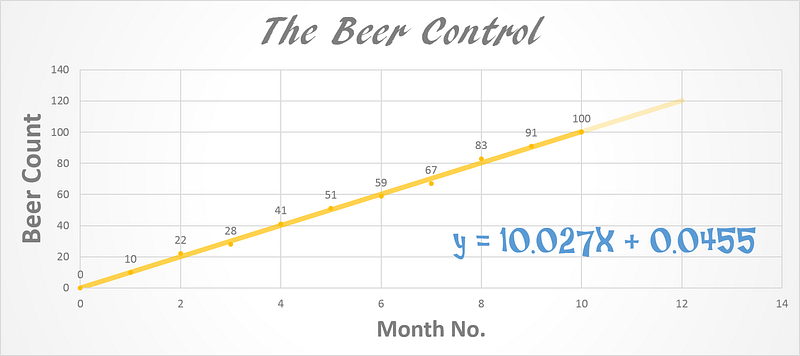
A simple linear regression shows what we could clearly see. Y = 10.027X + 0.0455 => m=10.027, c = 0.0455
c is a very small number so for now we will ignore it. Look at that the line equation tells us that for every month we drink 10.027 beers. That’s the trend. I derived this equation in MS PowerPoint but how can we do this mathematically?
How do machine learning engineers do this?
General Equation for Linear Regression
Bear with me. There is a slight bit of mathematics in this section but we will breeze right through it.
Linear regression is a form of supervised learning. Supervised learning involves those set of problems where we already have some data that can be used to predict new data. In the beer example we already know the data for the first 10 months. We just have to predict the data for 11th and 12th month.
Linear regression can involve multiple independent variables. e.g. house price (dependent) depending on both location (independent) and land area (independent) but in its simplest form it involves 1 independent variable.
In its generic form it is written as

where all the alphas are coefficients that our machine learning algorithm has to figure out. The x’s are known because they are independent. We can set them anything. What we need to find is Y.
For a single independent variable the equation is reduced to

For simplification x0 is set to be equal to 1 and alpha0 is given the name c. x1 is called x and alpha1 = m. It reduces to:
Jargon
To figure out m and c we draw a line (using an initial guess of m and c) through the set of points that we already have. We calculate the distance of this line from each of these points. We take square-root of the sum of the squares of these distances (Cost Function) . We keep changing m and c in small steps to see if this Cost Function decreases. When the cost stops decreasing we fix that m and c as our final result. The resulting line is our best linear fit through the data. Now for any new x we can figure out the y using this line.
That’s all the jargon that was needed. To make it more clear let me show you a few examples.
Manual Fit — Fitting a Line Manually To Data
Consider a data which has just three points. Listed in the (X,Y) format they are (1,2), (2,1) and (2,3).
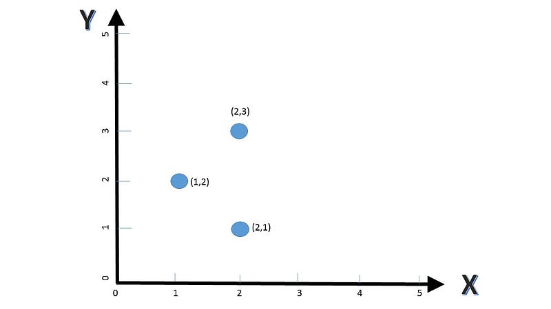
To make it simpler we will just consider shifting the line to three positions and based on that we will see which one to choose.
The three lines and their corresponding costs is shown below
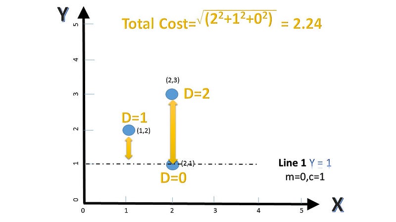
The second and third line and their respective costs
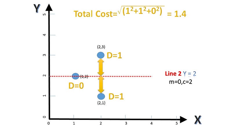
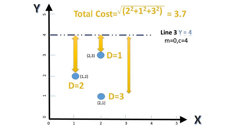
Line 2 has the least cost and fits our data the best. Line 2 is the winner yay!! This analytical analysis is fine as long as there are a couple of points. But for bigger datasets the cost function needs to be evaluated at small steps. One of the ways to evaluate that is called Gradient Descent, which is out of scope for the purposes of this article. I will unravel it in a future post (promise!).
Machine Learning — Auto fitting the line
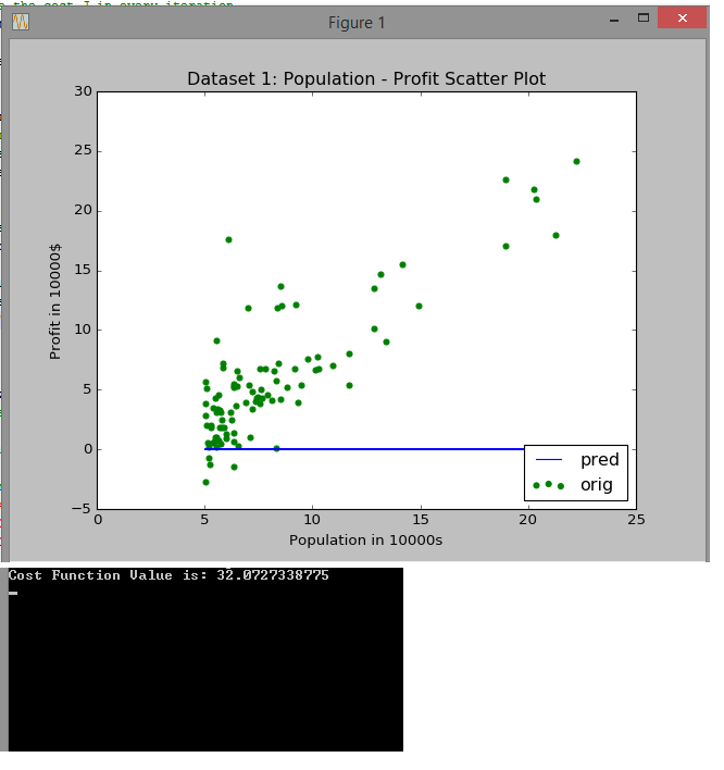
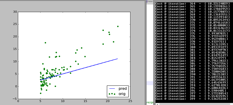
Below are the screenshots of a piece of code that I wrote to perform simple linear regression on a dataset given in a coursera assignment for a Machine Learning course taught by the famous Andrew Ng.
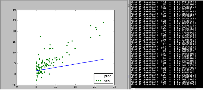
Look closely at how the initial guess (blue line) shifts towards the trend that the data follows. Also look at how many iterations are needed to reach that stable cost of 5.87
It starts with a cost of 32 and an initial guess way off!
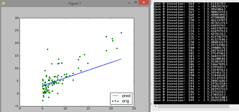
It steadily improves from then on. After 200 iterations the cost has already halved.
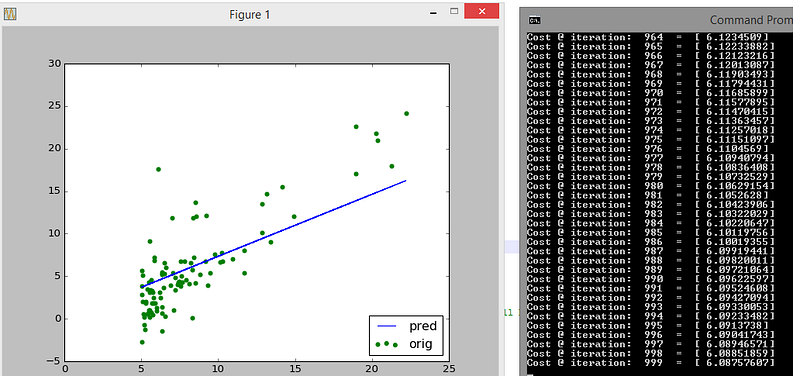
After 400 iterations the cost is 1/3rd
The guess improves further at 600 iterations
After a 1000 iterations the decrease in cost has slowed down and the fit is more or less stable
Just to verify the stability we check after roughly 3000 iterations
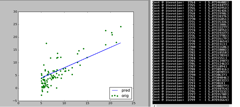
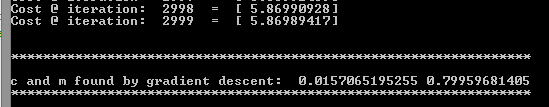
c and m are found out hence from this line as being equal to 0.02 and 0.8 respectively.
It is as simple as that! To be fair a simple line fit is more statistical modelling than machine learning. Linear regression becomes machine learning when Big Data is involved, when the number of explanatory variables (features) becomes much larger than what is used in statistical models, when significance of features takes a back seat and predictive power becomes important etc.
What is definite is that linear regression is a simple approach to predict based on a data that follows a linear trend. It follows that we will fail rather drastically if we were to fit a sine curve or a circular data set.
Finally, linear regression is always a good first step (if the data is visually linear) for a beginner. It is definitely a good first learning objective!
Resources
- Machine Learning by Stanford
- “An Introduction to Gradient Descent and Linear Regression” by Matt Nedrich
- “Linear Regression by using Gradient Descent Algorithm: Your first step towards Machine Learning” by Souman Roy
X8 aims to organize and build a community for AI that not only is open source but also looks at the ethical and political aspects of it. More such experiment driven simplified AI concepts will follow. If you liked this or have some feedback or follow-up questions please clap and comment below

Thanks for reading!