Summary

The article provides an in-depth exploration of Convolutional Neural Networks (CNNs), focusing on the architecture and functioning of layers, nodes, kernels, and the backpropagation process.

Abstract

This article builds upon foundational knowledge of CNNs to delve into the complexities of their architecture, particularly the roles of layers, nodes, and kernels. It categorizes CNN layers into input, hidden, and output layers, emphasizing the input layer's role in data preparation, hidden layers' feature extraction capabilities, and the output layer's production of predictions. The concept of nodes as computational units within feature maps is discussed, alongside the importance of kernels in feature detection. The backpropagation algorithm is detailed as a method for training CNNs by adjusting weights based on the loss function's output. The article also explains kernel stride and its impact on feature map size, providing practical examples to illustrate spatial downsampling. The author encourages reader interaction and promotes further learning through their book on machine learning.

Opinions

The author suggests that understanding the intricacies of CNN layers and their interconnections is crucial for grasping how CNNs process and transform data.
The article posits that hidden layers are where the core learning of a CNN occurs, as they contain the learnable parameters that capture data representations.
The author emphasizes the significance of the output layer, which not only produces the final prediction but also incorporates the loss function to measure the model's performance.
The article conveys the idea that backpropagation is an essential algorithm in neural network training, guiding the adjustment of weights to minimize the loss function effectively.
The author provides the opinion that by manipulating the kernel stride, one can control the compression of the feature map, which is a critical aspect of designing a CNN architecture.
The author believes in the practical value of their explanations and invites readers to engage with their content by following their work and considering their book for a comprehensive introduction to machine learning.

Going Deeper with CNN: Understanding Layers, Nodes, Kernels and Backpropagation

If you’ve come across this article while trying to understand Convolutional Neural Networks (CNNs), it would be beneficial for you to begin by reading my previous article:

https://readmedium.com/a-gentle-introduction-to-convolution-neural-networks-cnn-9455dfda49be

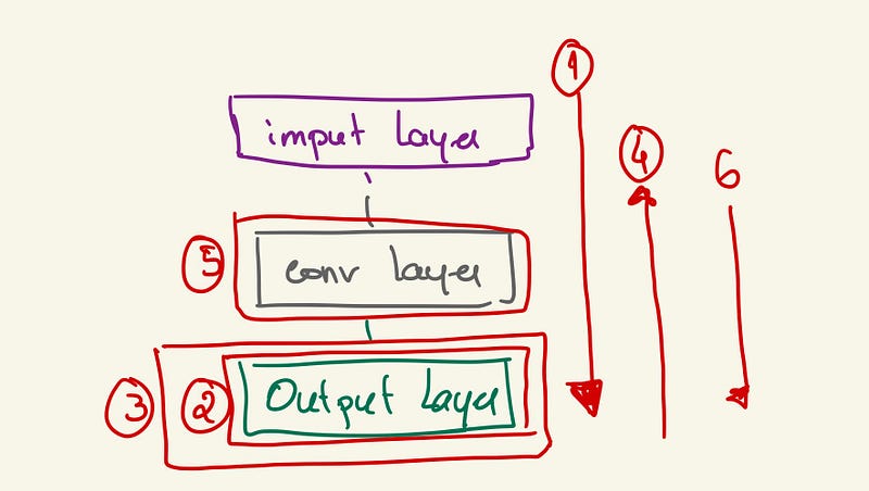
Now, let’s delve deeper into CNN by gaining a better understanding of layers and how they are interconnected and communicate. In general, there are three primary types of layers: (1) the input layer, (2) hidden layers, and (3) the output layer.

→ The Input Layer: serves as the entry point for the input data and prepares it for subsequent layers. This initial step may involve altering the data format and size to suit the network’s requirements. It’s important to note that the input layer is typically regarded as a data preprocessing layer and does not possess any learnable parameters.

→ Hidden Layers: refer to all the layers positioned between the input layer and the output layer. These layers are termed “hidden” because we cannot directly observe their outputs. It is within these hidden layers that the learnable parameters come into play and capture data representations. Think of the hidden layers as the layers responsible for extracting and transforming features from the data. A hidden layer receives information from the preceding layer and transmits information to the subsequent layer.

→ Output Layer: serves as the final layer in the network and produces a result or prediction based on the learnings acquired from the preceding layers. The output layer encompasses both the activation function, which introduces non-linearity to the output, and the loss function, which quantifies the discrepancy between the predicted output and the actual output.

You can learn more about Loss Functions here:

https://readmedium.com/10-commonly-used-loss-functions-explained-with-python-code-59967e1f3c8d

A convolution layer is a hidden layer!

Kernels, Feature Maps, and Nodes

In the previous article, we explored the concepts of kernels and feature maps and their relationship. Now, let’s take another step forward and delve into nodes. In CNN, nodes can be considered as the “neurons” within each feature map. Each node acts as a fundamental computational unit, performing calculations on the input it receives.

Backpropagation

Remember that the output layer can have a loss function? This loss function measures how well the model fits the data. Backpropagation is an algorithm used for training neural networks, which adjusts the weights of the network based on the output of the loss function. Now, let’s explore how it works by designing a very simple CNN schema:

Forward pass: An initial model is constructed, and its weights are saved.
Loss calculation: The loss function is utilized to calculate how well the model fits the data. It’s important to remember that the best model is the one in which the loss function is minimized.
Gradient calculation: The gradient of the loss function is computed. This gradient will guide the model in the descent direction, indicating how the weights should be adjusted.
Backward pass: Once the algorithm determines the gradient direction, the information is propagated backward through the network to guide weight updates in the correct direction.
Weight update: The model weights are adjusted to move closer to the minimum of the loss function.
Repeat: Steps 1 to 5 are iteratively repeated until either the loss function is sufficiently reduced or a tolerance level is reached. This iterative process is commonly referred to as an epoch.

Kernel Stride

The kernel stride determines the movement of the kernel across the input image. The stride value specifies the number of pixels by which the kernel shifts horizontally and vertically at each step. Once the kernel size and stride are known, we can calculate the output size or feature map size using the following formula:

Output size = ((Input size — Kernel size) / Stride) + 1

For example, if our input is an image of size 128x128, and our model has a kernel size of 11x11 and a stride of 2, the output size will be:

Output = ((128–11)/2) + 1 = 60

With a stride of 6, the output size is:

Output = ((128–11)/6) + 1 = 21

By adjusting the kernel stride, it is possible to control the spatial downsampling or compression of the feature map.

Let’s see another example: → With an image of size 128x128 in RGB format. Our input feature map will be 128x128x3 (where 3 is for the RBG format with its three-channel size). → Our convolution layer has 28 kernels, of size 6x6 and the stride is 4. To know the size of the output feature map we do ((128–6)/4)+1 = 32. → Since our convolution layer has 28 kernels, the size of the feature map obtained is 32x32x28.

Thank you for reading! Let me know if you have suggestions to add to this list, and don’t forget to subscribe to receive notifications about my future publications.

If: you liked this article, don’t forget to follow me and thus receive all updates about new publications.

Else If: you want to read more on topic, you can by my book “Data-Driven Decisions: A Practical Introduction to Machine Learning” that will give you all the information you need to start with Machine Learning. It will cost you only a coffee, and makes me a small tip!

Else: Thank you!