
10 Commonly Used Loss Functions Explained with Python Code
Understanding Loss Functions in Machine Learning

Table of contents:
What is a loss function?
Loss Functions vs Metrics
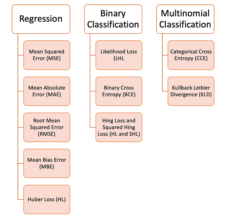
Why are loss functions applied while building the model?Regression:
Mean Squared Error (MSE)
Mean Absolute Error (MAE)
Root Mean Squared Error (RMSE)
Mean Bias Error (MBE)
Huber LossBinary Classification:
Binary Cross Entropy (BCE)
Hing Loss and Squared Hing Loss (HL and SHL)
Likelihood Loss (LHL)Multinomial Classification:
Categorical Cross Entropy (CCE)
Kullback-Leibler Divergence (KLD)What is a loss function?
A loss function is an algorithm that measures how well a model fits the data. A loss function measures the distance between an actual measurement and a prediction. This way, the higher the value of a loss function, the wronger the prediction will be. In contrast, a loss function with a lower value means that a prediction is closer to the real value. Loss functions are calculated for each individual observation (data points). The function that averages the values of all loss functions is called the Cost Function.
Loss Function: Calculates the error for each sample. Cost Function: Average of all loss functions.
Loss Functions vs. Metrics
Some loss functions are also applied as evaluation metrics. However, loss functions and metrics have different purposes. While metrics are used to evaluate the performance of the final model and to compare the performance of different models, loss functions are used during the model-building phase as an optimizer for the model under creation. Loss functions guide the model on how to minimize error.
Metrics: How well the model fits the data Loss function: How badly the model fits the data
Why are loss functions applied while building the model?
As loss functions measure the distance between predictions and real values, they are used while the model is building in order to guide the model in an improvement way (usually gradient descent — but I will talk about it in another article). This means that while the model is under construction if the feature’s weights are changed, we can have better or worse predictions. The loss function is used to tell the model with the feature’s weights that should be changed and the direction of that change.
There are a variety of loss functions that we can use in Machine Learning, depending on the type of problem we are trying to solve, data quality and distribution, and the algorithm we are using.
Regression Problems:
Mean Squared Error (MSE) Mean squared error finds the squared difference between all predicted values and the real values and averages it all. It is used for regression problems.
def MSE (y, y_predicted):
   sq_error = (y_predicted - y) ** 2
   sum_sq_error = np.sum(sq_error)
   mse = sum_sq_error/y.size
   return mse
Mean Absolute Error (MAE) This loss function is calculated as the mean of the absolute difference between predicted values and true values. This is a better measure than mean squared error when data has outliers.
def MAE (y, y_predicted):
   error = y_predicted - y
   absolute_error = np.absolute(error)
   total_absolute_error = np.sum(absolute_error)
   mae = total_absolute_error/y.size
   return mae
Root Mean Squared Error (RMSE) Is the squared root of the mean squared error. This is an ideal transformation if we don’t want to penalize larger errors.
def RMSE (y, y_predicted):
   sq_error = (y_predicted - y) ** 2
   total_sq_error = np.sum(sq_error)
   mse = total_sq_error/y.size
   rmse = math.sqrt(mse)
   return rmse
Mean Bias Erros (MBE) It is similar to mean absolute error but without applying the absolute function. The disadvantage is that negative and positive errors can cancel each other, so it is better applied when the researcher knows the error has only one direction.
def MBE (y, y_predicted):
   error = y_predicted -  y
   total_error = np.sum(error)
   mbe = total_error/y.size
   return mbe
Huber Loss The Huber Loss function combines the strengths of mean absolute error (MAE) and mean squared error (MSE). This happens because Hubber loss is a function with two branches. One branch is applied to MAE that fits under the expected values, and the other branch is applied to outliers. The Hubber Loss general function is:
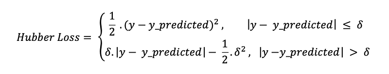
where:
- We already know how to find MAE from previous code examples.def hubber_loss (y, y_predicted, delta)
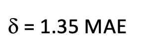
delta = 1.35 * MAE
y_size = y.size
total_error = 0
for i in range (y_size):
erro = np.absolute(y_predicted[i] - y[i])
if error < delta:
hubber_error = (error * error) / 2
else:
hubber_error = (delta * error) / (0.5 * (delta * delta))
total_error += hubber_error
total_hubber_error = total_error/y.size
return total_hubber_errorBinary Classification:
Likelihood Loss (LHL) This loss function is primarily used for binary classification problems. The output is a multiplication of the probability for the ground truth labels, and the associated cost function is the average for all observations. Let’s take the following example for binary classification, where categories are [0] or [1]. If we have an output probability equal to or higher than 0.5, then the predicted class is [1], otherwise is [0]. The example output probabilities are:
[0.3 , 0.7 , 0.8 , 0.5 , 0.6 , 0.4]
The corresponding predicted classes are:
[0 , 1 , 1 , 1 , 1 , 0]
The true classes are:
[0 , 1 , 1 , 0 , 1 , 0]
We will now use the true classes and output probabilities to compute likelihood loss. If the true class is [1], we use the output probability. If the true class is [0], we use 1-output probability:
Total cost = ((1–0.3)+0.7+0.8+(1–0.5)+0.6+(1–0.4)) / 6 = 0.65
You can also use the following code to compute likelihood loss:
def LHL (y, y_predicted):
   likelihood_loss = (y * y_predicted) + ((1-y) * (y_predicted))
   total_likelihood_loss = np.sum(likelihood_loss)
   lhl = - total_likelihood_loss / y.size
   return lhl
Binary Cross Entropy (BCE)
This function is a modification of the likelihood loss with logarithms. Adding the logarithms has the power to penalize predictions that are very confident and very wrong. The general formula for binary cross entropy loss function is:
— (y . log (p) + (1 — y) . log (1 — p))
Let’s try it with the values from the previous example:
Output probabilities = [0.3 , 0.7 , 0.8 , 0.5 , 0.6 , 0.4] True classes = [0 , 1 , 1 , 0 , 1 , 0]
— (0 . log (0.3) + (1–0) . log (1–0.3)) = 0.155 — (1 . log(0.7) + (1–1) . log (0.3)) = 0.155 — (1 . log(0.8) + (1–1) . log (0.2)) = 0.097 — (0 . log (0.5) + (1–0) . log (1–0.5)) = 0.301 — (1 . log(0.6) + (1–1) . log (0.4)) = 0.222 — (0 . log (0.4) + (1–0) . log (1–0.4)) = 0.222
Total cost = (0.155 + 0.155 + 0.097 + 0.301 + 0.222 + 0.222) / 6 = 0.192
def BCE (y, y_predicted):
   ce_loss = y*(np.log(y_predicted))+(1-y)*(np.log(1-y_predicted))
   total_ce = np.sum(ce_loss)
   bce = - total_ce/y.size
   return bce
Hinge Loss and Squared Hing Loss (HL and SHL) Hinge loss was primarily developed to evaluate SVM models. With Hinge loss, the wrong predictions and less confident right predictions are penalized. The general loss function is:
l(y) = max (0 , 1 — t . y)
where t is the true outcome [1] or [-1].
To apply Hinge loss, the classes should be [1] or [-1] (not [0]). In order to not be penalized in the Hinge loss function, an observation not only needs to be correctly classified, but the distance to the hyperplane should be larger than the margin (a confident right prediction). If we want to further penalize higher errors, we can square the Hinge loss value in a similar way that is used in MSE.
Remember that in SVM, the higher the margin for the hyperplane, the more confident is a certain prediction. You can recap SVM concepts in this article:

Now let’s see an example with visualization:
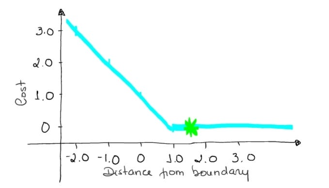
→ If a prediction has an outcome of 1.5 and the true class is [1], the loss will be 0 (zero) because the model is highly confident.
loss = max (0 , 1–1* 1.5) = max (0 , -0.5) = 0
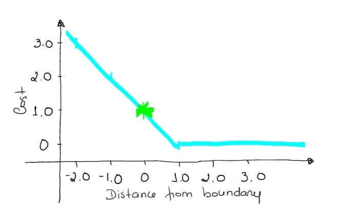
→ If an observation has an outcome of 0 (zero), it means that the observation is in the boundary (hyperplane), and the true class is [-1]. The cost is 1, the model is neither wrong nor right, and it has very low confidence.
loss = max (0 , 1–(-1) * 0) = max (0 , 1) = 1
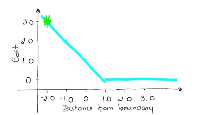
→ If an observation has an outcome of 2, but it is wrongly classified (multiply by [-1]), we have a distance of -2. The cost is 3 (very high), because our model is very confident in a wrong decision.
loss = max (0 , 1 — (-1) . 2) = max (0 , 1+2) = max (0 , 3) = 3
#Hinge Loss
def Hinge (y, y_predicted):
   hinge_loss = np.sum(max(0 , 1 - (y_predicted * y)))
   return hinge_loss
#Squared Hinge Loss
def SqHinge (y, y_predicted):
sq_hinge_loss = max (0 , 1 - (y_predicted * y)) ** 2
total_sq_hinge_loss = np.sum(sq_hinge_loss)
return total_sq_hinge_lossMultinomial Classification:
Categorical Cross Entropy (CCE)
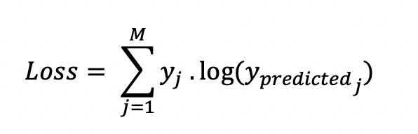
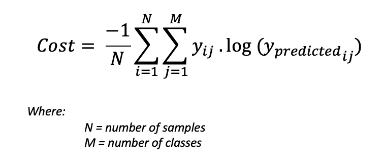
In multinomial classification, we use a similar formula as in the binary cross entropy, but with one extra step. W first need to calculate the loss for every single pair of [y , y_predicted], and the general formula is:
If we have a three-class problem, where the output of a single [y , y_predicted] pair is:
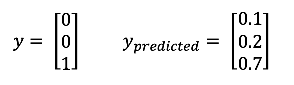
The true class is 3, and our model is 0.7 confident that the real class is 3. To calculate the loss for this single pair:
Loss = 0 . log (0.1) + 0 . log (0.2) + 1 . log (0.7) = -0.155
To get the value for the cost function, we need to compute the loss for all individual pairs, sum all of them, and finally, multiply by [-1/number of samples]. The cost function is given by the following formula:
Using the above example, and if we have a second pair:
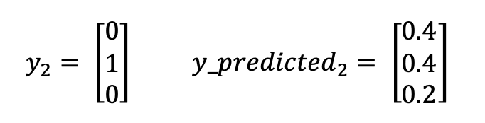
Loss = 0 . log (0.4) + 1. log (0.4) + 0. log (0.2) = -0.40
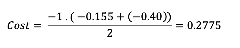
The cost function will be calculated as:
It can be easier to understand using the code example:
def CCE (y, y_predicted):
   cce_class = y * (np.log(y_predicted))
   sum_totalpair_cce = np.sum(cce_class)
   cce = - sum_totalpair_cce / y.size
   return cce
Kullback-Leibler Divergence (KLD) Similar to categorical cross entropy, but also takes into account the probability of occurrence of the observations. It is particularly useful if our classes are not balanced.
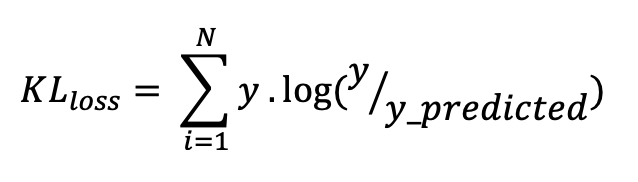
The code is:
def KL (y, y_predicted):
   kl = y * (np.log(y / y_predicted))
   total_kl = np.sum(kl)
   return total_kl
Thank you for reading! Don’t forget to subscribe to receive notifications about my future publications.
If: you liked this article, don’t forget to follow me and thus receive all updates about new publications.
Else If: you want to read more on the topic, you can buy my book “Data-Driven Decisions: A Practical Introduction to Machine Learning” which will give you all the information you need to start with Machine Learning. It will cost you only a coffee, and give me a small tip!
Else: Thank you!


