DATA SCIENCE, OPTIMIZATION, PROGRAMMING

Genetic Algorithm — Stop Overfitting Trading Strategies

How can the Coefficient of Variation make Genetic Algorithms more robust?

In a previous blog, we have talked about how the Genetic Algorithm can be used for optimizing parameters of a trading strategy, and hence parameters of any non-linear functions given an appropriate fitness/cost function. The arguably most important part that we have not touched on, is how do we make sure that the GA is well-fitted but not overfitted.

This time, we will be going through how to ensure a robust GA training process when applied to a time series problem using the same MACD strategy as an example. If you have not read my blog on how to apply a Genetic Algorithm to trading strategy optimization, I would strongly encourage you to either skim through the tutorial or go through the full script here on GitHub as this blog will pick up from where we left off.

Note: We will be covering the code section by section. If you find it hard to follow or glue them together, don’t worry! Link to the full script is at the end of the blog.

Another Note: This is only a demonstration of how to avoid overfitting a GA when optimising a trading strategy and is not intended to be followed blindly.

Quick Intro to Genetic Algorithms

Darwin-inspired iterative heuristic searching algorithm for the global optimal solution, also known as Genetic Algorithm. It represents a candidate solution (individual) as a list of parameters (genes). How successful an individual (fitness value) is determined by a fitness function. The probability for the solution to reproduce in general follows “survival of the fittest” (selection strategy). The fittest solutions then reproduce the children (crossover), the grandchildren, and the grand-grandchildren. Some generous of mutation in the solution parameters are also sprinkled in so that fish can finally evolve into humans who can run another Genetic Algorithm.

So that’s a very condensed crash course on how Genetic Algorithms work in an analogy. If you are interested in each of the concepts, I have written a more detailed crash course on what each component means.

Overfitting in Genetic Algorithms

Bear with me, this is not yet another paraphrased definition of overfitting. Instead, we are going to briefly talk about a specific type of overfitting for GA or Neural architecture search (NAS):

Bloating: This is a phenomenon where a parameter/hyperparameter optimization algorithms like GA decides to use a very complex solution to achieve marginal gains in fitness. As GA has been given the freedom to compete with itself within a set number of iteration, the complexity of the final solution can grow uncontrollably and become so overfitted to the noise that it will be nothing but an incomprehensibly complex yet useless black box.

In recent years, a technique called Random Subset Selection (RSS) has been developed to both speed up the training process of a Genetic Algorithm, and to reduce overfitting of it. The intuition behind is simple:

If a solution performs consistently well across a number of subsets of the population, it is likely to be more applicable in unseen data.

Various branches of RSS has been discussed in several research papers and applied onto some well know open datasets like Toxicity, Bioavailability etc, each with a slight twist to how it can be further improved, but there has been one thing in common that makes it less applicable to us:

1. Our problem statements are not strictly classification problems: Unlike their datasets, ours do not have a constant label/classification. In fact, the result of our underlying problem is a cumulative product of the percentage returns of the trades; and whether a trade is profitable solely lies with the entry and exit strategy.
2. Our solution space has a consistent complexity of 3 parameters: Although our underlying problem sounds more complex than theirs, our solution is actually not. Unlike trying to come up with a protein chain that can crack COVID-19, or build a multi-layer forest model to classify toxicity of a compound, our solution for a MACD strategy has and only has 3 parameters: fast, slow, and signal period.

Extending RSS: Coefficient of Variation

The core concept of RSS is to find solutions that are consistent across slices of the dataset, rather than just the entirety of it. If we break that sentence down, there are two things that we need to keep in mind:

• Slicing sizeable set(s) for training — There is no point in evaluating trading performance in 1 day when a round trip for our MACD strategy takes a month or two to close.
• Low variance in performance — A good strategy needs to weather both bullish and bearish runs.

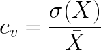
To combine these two concepts, we can leverage a statistical concept called the coefficient of variation (CV), which we can simply calculate as the ratio between the standard deviation and the mean of fitness values from some random slices of the training set. CV is also called deviation risk measure in financial mathematics and unitized risk in actuarial sciences.

The higher the coefficient of variation, the higher the deviation and risk a trading strategy bears

Note: CV should be computed using ratio-scale data instead of absolute value (e.g. absolute profit) or interval-scale data (e.g. degree Celcius). Such data should have an absolute zero which allows a meaningful measurement of ratios (e.g. 20K is twice as hot as 10K)

Now that we have got all the core concepts for this blog post covered, let’s dive straight into the code!

1. Quick Recap

In the previous blog post, we have developed our MACD Strategy and Genetic Algorithm Parameter Optimisation with alphavantage, backtrader and deap. The underlying dataset that we have downloaded from alphavantage is the daily candlesticks of NVDA. Our Genetic Algorithm has the following configurations:

• Genes: Parameters for our MACD Strategy are fast_period, slow_period, and signal_period
• Initial Population: Our initial population will have 100 individuals, each with random integers fast_period in the range of [1, 151), slow_period in the range of [10, 251), and signal_period in the range of [1, 301)
• Fitness function: Total Profit / Maximum Draw Down of the MACD strategy
• Selection Strategy: Tournament method where the winner of each round of the tournament will be selected as the seeds for the next generation
• Crossover Strategy: We will be using uniform crossover with a 50% chance for each gene to crossover
• Mutation Strategy: We will be using a uniform distribution of integers in the range of [1, 101) with a mutation probability of 30% for each gene
• End Conditions: The algorithm will stop once it has finished 20 iterations

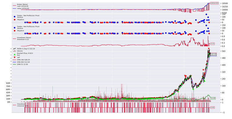
The optimal solution that we have obtained is fast_period=36, slow_period=84and signal_period=5 with a Total Profit / Maximum Draw Down of 5.33, and a total profit of 518.85 USD.

2. Separate Training and Testing Set

To stop our genetic algorithm from getting too good at playing with the training set that the knowledge it acquired cannot be generalized and applied onto unseen data, let’s first change the data loading script and create a testing set which the algorithm will not be trained on. This testing set will act as a final exam for us to check if the results can be applied in the future:

# let's look at how many rows of data we have got
df = read_alpha_vantage(ticker=TICKER)
print(df.shape, df.index.min(), df.index.max())

(5327, 5) 1999-11-01 2020-12-31

# let's keep 4 years of testing data
TRAIN_TEST_SPLIT_DATE = datetime.datetime(2017, 1, 1)
df_train = df[df.index < TRAIN_TEST_SPLIT_DATE]
df_test = df[df.index >= TRAIN_TEST_SPLIT_DATE]
print(df_train.shape, df_train.index.min().date(), df_train.index.max().date())

(4320, 5) 1999-11-01 2016-12-30

print(df_test.shape, df_test.index.min().date(), df_test.index.max().date())

(1007, 5) 2017-01-03 2020-12-31

# this training set is all that the algorithm will use
data = bt.feeds.PandasData(dataname=df_train, name=TICKER)

3. Coefficient of Variance as a Fitness Function

With the new benchmark established, it’s time to change the meat inside. To incorporate CV into our fitness function, we will need to first add 2 hyperparameters to our fitness function:

• n: Number of random slices of training data
• l: Length of a random slice

Note: Unlike parameters, hyperparameters would not increase our solution complexity in this case.

We will also need to adjust the way the fitness value is calculated. Recall that CV works only if the underlying measurement is ratio-scale-based and has a meaningful 0. This means that we can no longer use our original fitness function Total Profit / Maximum Draw Down as it does not have an absolute zero. Instead, we will update it to Final Value / (Initial Capital * (1 — Maximum Percentage Draw Down)). As backtrader does not allow negative equity, when fitness value is zero, that literally means we have lost everything and cannot be worse, i.e. that can be used as an absolute zero.

Let’s say we set n to 10 and l to 0.2. What that means is our fitness function will now draw 10 continuous samples with 20% the size of the entire training set each. It will then calculate the new fitness value as the CV of our new metric, f as shown below.

Another thing to be noted when slicing the training set is that the training set needs to be at least as long as the largest parameter. For example, if our fast_period is 15 days, then the slice needs to be at least 16 days for any valid signal to happen. To avoid insufficient data in the slice of the training set, let’s define slice_length = int(len(df_train) * l + max(parameters)) such that each slice will now be of length slice_length. This way we will make sure that each slice will have a trading window of the same length. Our new evaluate now looks like this:

4. Evaluation

With the new fitness function, we can then plug it back into the script that we have been using in the last blog post for running GA:

After running the snippet, we have the following results

HALL OF FAME:
    0: [136, 145, 150], Fitness: 0.010034400410587742
    1: [136, 145, 138], Fitness: 0.00872738799658447
    2: [135, 136, 138], Fitness: 0.008081687727270134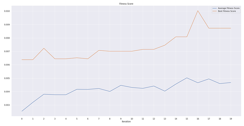

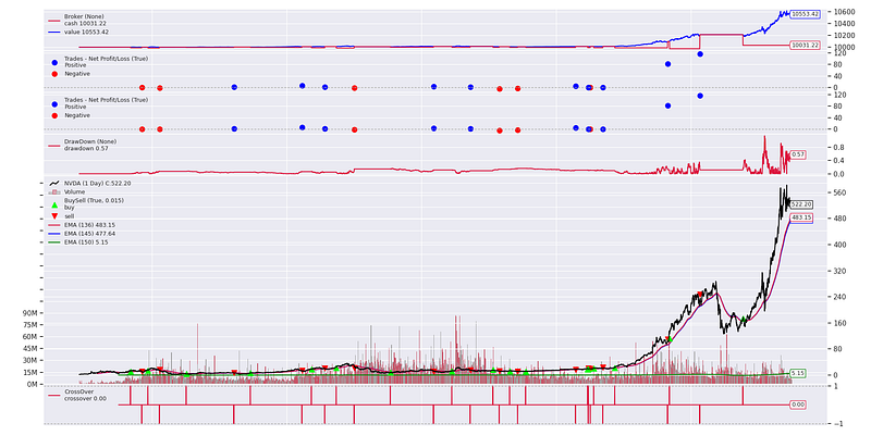
• Comparable performance with a smaller set of training data: Training with 90% of data and with random sample subsets, our new GA has identified a way longer-term strategy which ends up a better profit than before.
• Less scalping, less trading cost: Compared against the strategy before with fast_period=36, slow_period=84and signal_period=5, our new strategy with fast_period=136, slow_period=145and signal_period=150 has way fewer entry signals. As a result, we are paying less on trading fee.
• Out-performing HODLing: This is always welcoming news. Rule of thumb: if a strategy is worse than buy and hold, then that’s not a viable strategy at all.

5. Closing Thoughts

In this blog, we have looked into how we can tweak a Genetic Algorithm to make it more robust with Coefficient of Variation and Random Subset Selection. We have managed to achieve a better final result with 81% of our entire dataset. However, this is by no means the golden ticket to parameter optimization with Genetic Algorithms. Here are some extra ideas that you may want to look into:

• Understanding data bias: This can lead to very serious overfitting. For example, if the overall market is bullish, it makes sense that the GA is giving you good results, even if it just HODL. Imagine if you do the same when the market goes bearish.
• Statistical representativeness: If the test set is statistically different from the train set, what you may want to do is to add a validation set, which needs to be statistically similar to the test set. The training process would then need to consider both the fitness value in the train set and the test set.
• Multiple objectives: Instead of combining metrics as ratios as we have done in this blog, we can keep them as separate fitness values and have deap weight them differently. This may make our GA more interpretable if we want to add more metrics for the GA to optimize. But remember, adding more metrics may come at the price of overfitting.
• Expand our training set: This is almost the most common answer to any machine learning problem. But a couple of things to bear in mind — (1) While it is generally a good idea to mix up the statistical distribution of the training set a bit so that the algorithm is exposed to different scenarios, we still need to make sure that the training, validation, and testing set are still somewhat relevant, and (2) going back to the first closing thoughts, you should not risk biasing your training set too much just so that you can have a larger training set.

That’s about it for this blog post! As promised, here is the full script. I hope you have found this useful. If you want to learn more about Python, Data Science, or Machine Learning, you may want to check out these posts:

• 7 Easy Ways for Improving Your Data Science Workflow
• Efficient Conditional Logic on Pandas DataFrames
• Memory Efficiency of Common Python Data Structures
• Parallelism with Python
• Essential Jupyter Extension for Data Science Set Up
• Efficient Root Searching Algorithms in Python

References:

• Gonçalves, Ivo, and Sara, Silva. “Experiments on controlling overfitting in genetic programming.” Proceedings of the 15th Portuguese Conference on Artificial Intelligence: Progress in Artificial Intelligence, EPIA. Vol. 84. 2011.
• Langdon, W. B. “Minimising testing in genetic programming.” RN 11.10 (2011): 1.
• Gonçalves, Ivo, et al. “Random sampling technique for overfitting control in genetic programming.” Genetic Programming. Springer Berlin Heidelberg, 2012. 218–229.
• Gonçalves, Ivo, and Sara, Silva. Balancing learning and overfitting in genetic programming with interleaved sampling of training data. Springer Berlin Heidelberg, 2013.
• Gonçalves, Ivo, and Sara, Silva. “Experiments on controlling overfitting in genetic programming.” Proceedings of the 15th Portuguese Conference on Artificial Intelligence: Progress in Artificial Intelligence, EPIA. Vol. 84. 2011.
• Žegklitz, Jan, and Pošík, Petr. “Model Selection and Overfitting in Genetic Programming: Empirical Study.” GECCO Companion ’15: Proceedings of the Companion Publication of the 2015 Annual Conference on Genetic and Evolutionary Computation. Association for Computing Machinery, 2015. 1527–1528.