From Basic to Intermediate SQL in 10 Minutes

Table of Contents

• Basics - SELECT, WHERE, ORDER BY - WHERE details - Strings & Dates
• Intermediate - Aggregation - Aggregation filtering - Joins - Unions

Introduction

If you need a more general introduction to SQL and Databases, check out the first part of this tutorial:

In this article, we will look at basic SQL syntax; selecting data from tables, filtering and working with data types. We will then look at Joins and aggregate measures.

The syntax in this article is all you really need to work with data in SQL competently. Anything else just makes life easier.

SQL for Data Science — why?

SQL remains one of the most important skills for all data related roles in 2020. Regardless of the advances and uptake in NoSQL databases, companies still use relational databases widely and SQL is essential to extract data out.

Having SQL syntax at your fingertips ensures you are able to get data fast, understand complex databases quickly and spend more time on analysis. Using SQL to filter and roll up data before bringing it into another tool is especially helpful when working with very large datasets.

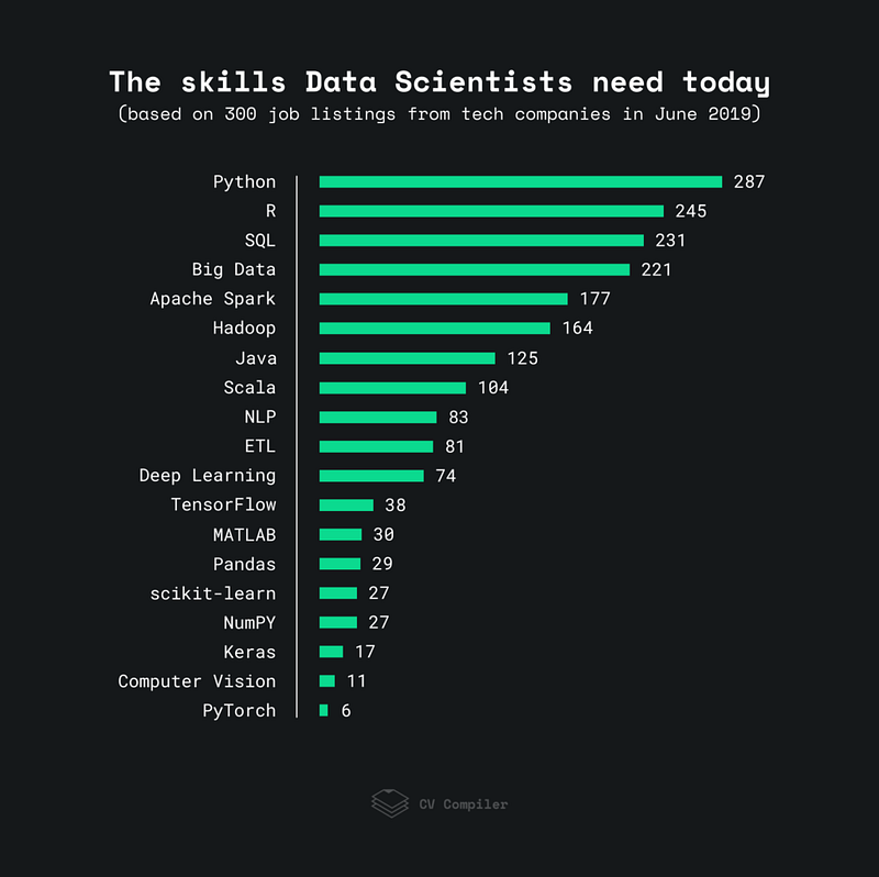
We can see from the below chart that SQL is consistently one of the most requested skills in job listings and many companies will test for SQL as part of their interview process.

Using SQL

SQL Best Practice

There are multiple different SQL database management systems. These have slightly different syntax and are provided by different vendors. Generally, there is a lot of equivalence between them so learning the fundamentals in one is highly transferrable. The main names you’ll hear are MySQL, PostgreSQL, MS SQL Server.

Best practice is to put syntax such as SELECT into capital letters, separate columns on new lines and indent after joins. You’ll see me use these however, SQL doesn’t need these formatting steps to work.

This tutorial uses SQLite and an Avocados dataset. If you want to build this yourself in under 5 minutes, take a look here.

Basics — SELECT, WHERE, ORDER BY

Exploring the data

Let’s take a quick look at the table before we filter it.

• SELECT * selects every column in the table.
• LIMIT 50 means we only get the first 50 rows.

SELECT *
FROM avocados
LIMIT 50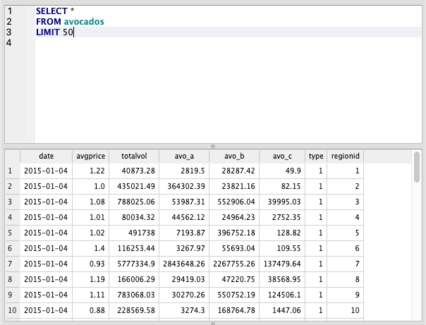

SELECT, WHERE, ORDER BY

We’re going to tackle these in one query.

The order of functions is essential in SQL. The order shown in these queries is generally the only order that works

SELECT 
   date
 , avgprice
 , totalvol
FROM avocados
WHERE type = 1
ORDER BY totalvol DESC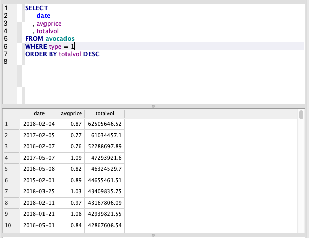

SELECT

• Here we define our columns via a comma separated list.
• We can use * to select all columns in the table.

FROM

• Here we define the table we want to pull the data from.
• In this case, the name of the table is avocados.

WHERE

• This is a filter. We can filter by any column in the table even if we haven’t selected it.
• Multiple filters can be chained together using AND/OR.

ORDER BY

• This sorts our data by the specified column.
• We can specify ASCending or DESCending afterwards to change the order.

Using WHERE

Comparison Operators

• We can use typical comparison operators with WHERE such as equals, greater than, less than etc.
• These are standard symbols. You can see a full list here.

Contains

• We can also use LIKE to find strings that contain a word.
• We combine LIKE with a percent symbol to specify anything after or anything before.
• The below query selects anything starting with ‘A’. We could put the percent sign before to find anything ending with ‘A’ (case-sensitive) or on both sides to find anything containing this character.

SELECT * 
FROM region
WHERE region LIKE ‘A%’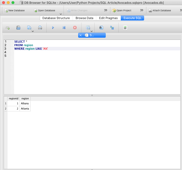

Filtering with a list

• One of the most commonly used functions with WHERE is IN which allows you to pass a list of items to filter by.
• In the example below, we treat date as a string and pass 2 dates to filter.
• We also combine this with a regionid filter.

SELECT *
FROM avocados
WHERE date IN ('2015-01-04','2015-01-11')
AND regionid=1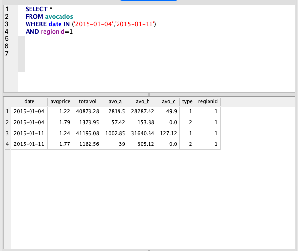

Working with Strings and Dates

Strings

String and Date syntax can vary a lot depending on which database management system you are using. In general, most of the string and date operations you can do in Excel are transferable to SQL but with different syntax.

SELECT 
   UPPER(region)
 , SUBSTR(region,2,5)
 , SUBSTR(region,-3,3)
FROM region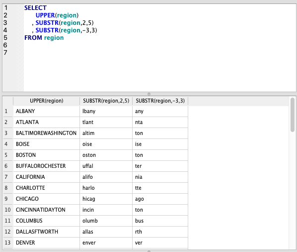

UPPER

• This converts the text to uppercase.
• This is very useful when used in conjunction with WHERE clauses if you are searching for a single word in text that is a mixture of cases.

SUBSTR

• This takes a subsection of the string using the numbers we specify, the first indicates the character to start on and the second is the number of characters we take.
• We can also use negative numbers to get the last characters.

For more information on strings, try: https://www.geeksforgeeks.org/sql-string-functions/

Dates

When working with dates, the key is to make sure your data has the correct data type; it should be stored as an actual date.

If it isn’t you’ll need to either talk to your database administrator and get them to update the ‘create table’ statement to convert this.

In SQLite we can’t work with dates as easily, but the Syntax below will work in Postgres.

SELECT my_date,
 EXTRACT(‘year’ FROM my_date) AS year,
 EXTRACT(‘month’ FROM my_date) AS month,
 EXTRACT(‘day’ FROM my_date) AS day,
 EXTRACT(‘hour’ FROM my_date) AS hour,
 EXTRACT(‘minute’ FROM my_date) AS minute,
 EXTRACT(‘second’ FROM my_date) AS second,
 EXTRACT(‘decade’ FROM my_date) AS decade,
 EXTRACT(‘dow’ FROM my_date) AS day_of_week
FROM table_name

If in Postgres, you can also use the DATE_PART function

SELECT DATE_PART(‘year’, my_date) AS year 
FROM table_name

Intermediate SQL — Aggregation, JOIN, UNION

Aggregation — SUM, AVG, MIN, MAX, GROUP BY

Let’s aggregate the data using the type column. We have 2 types, which at the moment are called ‘1’ and ‘2’. We’ll find out what those mean later.

The order is also very important here. The GROUP BY must go at the end, and if we are using a WHERE, this should go before the GROUP BY.

SELECT 
   type
 , AVG(avgprice)
 , SUM(totalvol)
FROM avocados
GROUP BY type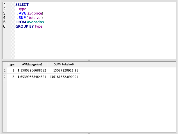

AVG

• This takes the average of the column in brackets by row

SUM

• This takes the sum of the column in brackets by row

These aggregate functions are calculated over the rows selected which means we need to group the rows to get to what we want — the average or sum by type

GROUP BY

• This is the column we want to group by.
• SQL is performing the AVG or SUM calculation on all the rows within a group based on this function.

Other commonly used aggregations are MIN, MAX, COUNT.

Aggregate Filtering

Let’s say we want to take our previous example and filter out the types where the avgprice is less than 1.5.

Obviously there are only 2 types here so we could do this by eye but imagine we had hundreds!

We’ve already learnt to filter using WHERE but this won’t work to achieve what we want.

We can’t use WHERE with aggregate functions such as SUM and AVG because this will filter the underlying rows, not our summarised data.

Filtering the underlying data means we actually filter the individual rows and not our summary table. See the example below.

If we use WHERE, the AVG and SUM are now calculated using only rows with avgprice > 1.5.

Enter HAVING. This allows us to filter the aggregated rows after they’ve been calculated.

SELECT 
   type
 , AVG(avgprice)
 , SUM(totalvol)
FROM avocados
GROUP BY type
HAVING AVG(avgprice) > 1.5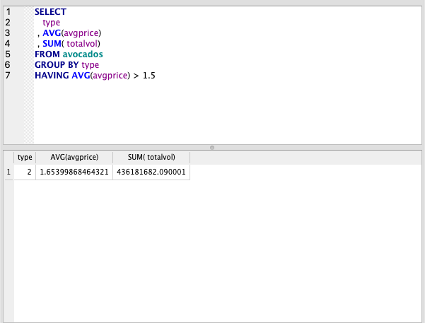

JOIN Theory

JOIN might be the single most important function in SQL. Understanding how joins work, in my opinion, takes you from a beginner to intermediate SQL user.

In order to understand joins, you should understand the basics of relational databases and STAR schema tables. The first part of this guide gives a good explanation.

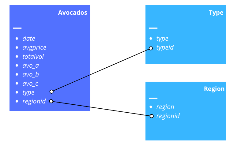
This is the schema of our set of tables. Without making joins we can’t get the actual type or region names because our Avocados table uses IDs in place of the actual names.

There are 4 main types of join; Inner, Outer, Left and Right. The differences are the rows that are kept in the joined table once the join is made.

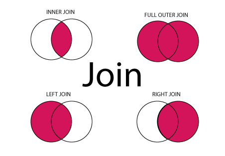
• INNER JOIN: Returns all rows where there is at least one match in BOTH tables.
• LEFT JOIN: Returns all rows from the left table and matched rows from the right table.
• RIGHT JOIN: Returns all rows from the right table and matched rows from the left table.
• FULL JOIN: Returns all rows where there is a match in ONE of the tables.

Consider a situation where a table has missing rows — eg if our Region table above was missing some region ids that were present in the main Avocado table.

In this situation, an INNER JOIN would cause us to lose any rows without a corresponding region id, so here we might want to use a left, right or outer join to keep all rows in the Avocado table.

It’s also worth noting that if there are duplicates in your dataset with the same ID, joining these will cause multiple lines to be created.

Making sure you understand duplicates in your data is one of the key things to be careful of when making a join.

JOIN Composition

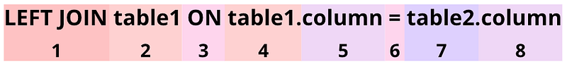
1. Specify the join type
2. Specify the table you are bringing on
3. After the ON, we name the columns
4. The order here doesn’t matter, if doing a LEFT JOIN, the left table is always the original table. The table you are bringing in is always the right table.
5. Specify the column
6. We put an equals sign between each column
7. This is the table you are joining to
8. This is the columns we are joining on. It should be equivalent to the table in ‘table1’ eg the same id.

You can use AND to join on multiple columns.

JOIN in SQL

We’ll just use left joins for the tutorial, but if you are following along, feel free to experiment with other join types.

SELECT *
FROM avocados
LEFT JOIN avo_type ON avocados.type = avo_type.typeid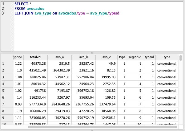

We now have the columns typeid and type from the avo_type table. Let’s select only the date, avgprice and type columns.

Take a look at the query below, we’ve changed 2 parts of this query.

First, we’ve specified exactly which columns we’ll be using.

Then, tables have been given aliases.

In SQL aliases are used to give a table, or a column in a table, a temporary name. Aliases are often used to make column names more readable. An alias only exists for the duration of the query.

We’ve called the avocados table ‘av’ and the avo_type table ‘avt’. We’ve also used these as an easy way to specify which columns to select. You’ll notice the type column is in both tables, so specifying which type we want is essential here.

SELECT 
   av.date
 , av.avgprice
 , avt.type
FROM avocados av
LEFT JOIN avo_type avt ON av.type = avt.typeid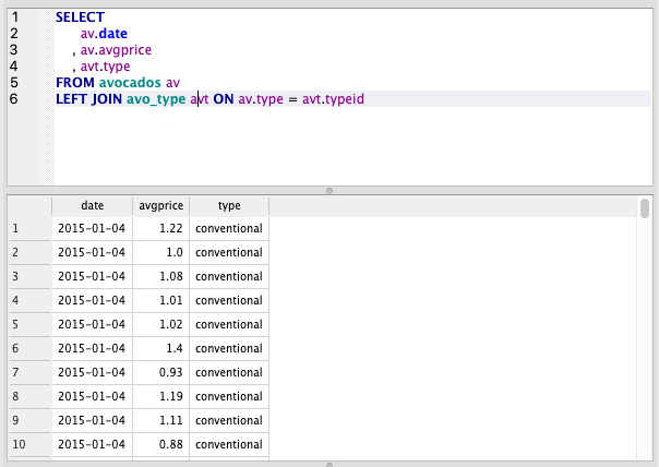

UNION

Unions are used when we want to put one table on top of another. It isn’t really applicable for the data we have in this example, but I’ll show the syntax anyway.

In this query, we filter to type =1 and then use a union to stack this on top of a table for type !=1

Note that we’ve renamed the sum column here but the UNION still stacks it as it uses the position of the column and not the column name.

SELECT type, sum(totalvol) as totalvol
FROM avocados av
WHERE type = '1'
UNION
SELECT type, sum(totalvol) as t
FROM avocados av
WHERE type != '1'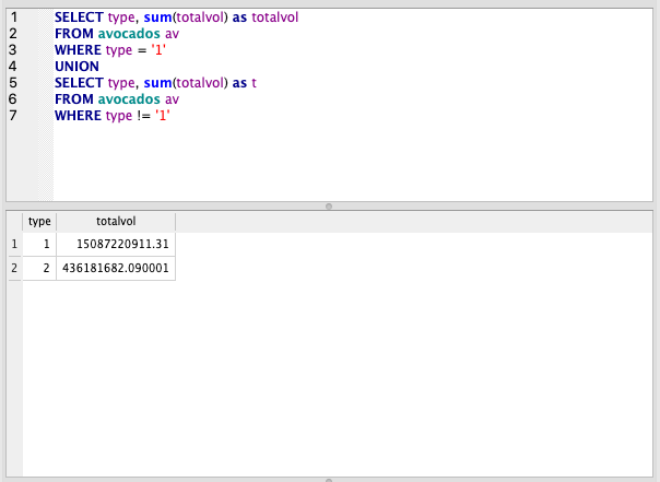

Summary

If you got to the end of this article, congratulations! You now have the required to knowledge to use SQL to a working standard.

Honestly, it doesn’t get much more complicated than this. Getting all the functions in this article mastered will ensure you can pass most SQL tests.

More SQL Articles:

Contact Me: