Advanced SQL for Data Scientists

Introduction

This article looks at a few techniques that if mastered, equips the user with the tools to deal with a wide range of data types. This article does not cover anything relation to database management such as table creation or schemas.

If you’d like to follow along, you can set up a local SQL Server using SQLite :

If these techniques are too complex, you can get up to speed in less than 10 minutes here:

Table of Contents

• Exploring the Example Data
• JOIN as a Filter
• Self Joins
• CASE WHEN
• Subqueries
• Common Table Expressions
• Window Functions - Running Total - Total by date - Moving Average - Get First Row

Exploring the Example Data

Let’s take a quick look at the table before we filter it.

SELECT *
FROM avocados
LIMIT 50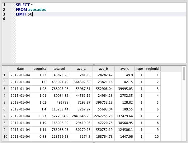

There are also 2 mapping tables in this dataset for type and regionid which map these numeric categories to their actual text.

JOIN as a Filter

By combining an INNER JOIN with a filter using AND, we can filter the table as we are joining it, providing a small performance boost over a regular join and WHERE filter. The is handy for big datasets but you’ll need to to know your data well as you may drop rows you didn’t intend to because this technique uses the INNER JOIN.

SELECT *
FROM avocados a
INNER JOIN region b ON a.regionid = b.regionid
AND b.region = 'Denver'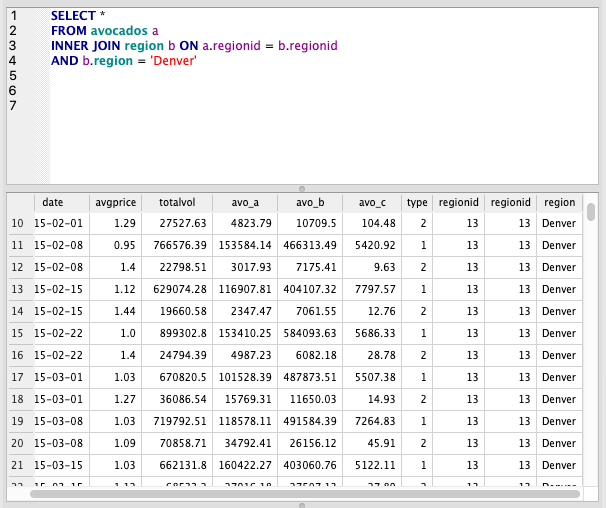

Self Joins

Self joins are particularly useful when we need information in different rows to be in the same row. My dataset isn’t exactly set up to do this but we can still illustrate the point.

Let’s try to get the total volume for 2 regions on the same date on the same row.

First, note the aliases we’ve given to each avocados table. It’s the same table, but we’ve called each one a and b.

Inside the join, we’ve joined on date and regionid but we’ve used the does not equal operator (<>) to ensure we don’t join the same types together.

The result is a single row with both types on it, instead of each appearing in separate rows.

Please note, we do end up with duplicate data here as we have every combination of types. This could be avoided by filtering.

SELECT 
  a.date, a.avo_a, a.type, 
  b.avo_a, b.type, b.regionid
FROM avocados a
INNER JOIN avocados b 
  ON a.date = b.date 
  AND a.regionid=b.regionid
  AND a.type <> b.type 
WHERE a.date = '2015-01-04'
  AND a.regionid = 1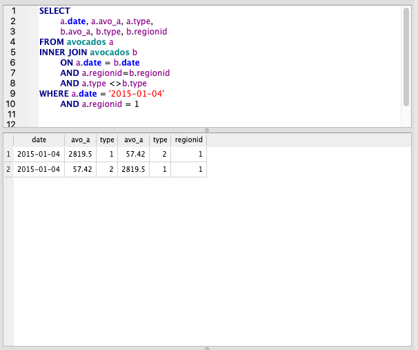

CASE WHEN

CASE WHEN is essentially an IF function, which is found in almost all coding languages. As always, remember the ‘flow’: IF -> THEN -> ELSE when writing these.

We’ll use this to map types to the actual types (we could also do this with a join to our types table).

Note that the formula starts with CASE and ends with END. We can give the column an alias using AS after the END.

We can have as many WHEN/THEN clases as needed. Here we only need one because we have 2 types and the 2nd is covered by the ELSE

SELECT date, avo_a,
 CASE
  WHEN type =1 THEN 'conventional'
  ELSE 'organic'
 END AS avo_type
FROM avocados
WHERE regionid = 1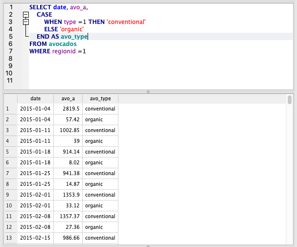

Subqueries

A subquery is a nested query; it’s a query within a query

Let’s say we want the full dataset but only for the top 10 regions by total volume.

We could find the top 10 with the query below, then we could use this list of regions to filter the main table. But what if we got new data and the top 10 changed? We’d have to run both queries again. We can make this more dynamic using a subquery.

To get the top 10, we’d run something like this:

SELECT b.region, ROUND(SUM(a.totalvol))
FROM avocados a
LEFT JOIN region b ON a.regionid=b.regionid
GROUP BY 1
ORDER BY 2 DESC
LIMIT 1

In the query below, we use an INNER JOIN to filter the list to the regions in the subquery. We can also bring back data from the subquery because we’ve joined it.

Please note how aliases work here. The subquery aliases are independent of the main query aliases, which is why we have 2 ‘a’ and ‘b’ aliases. To refer to subquery columns we have to use the subquery alias which is c in this case.

SELECT date, totalvol, avo_a, avo_b, b.region, c.total_totalvol
FROM avocados a
LEFT JOIN region b ON a.regionid=b.regionid
INNER JOIN (
  SELECT b.regionid, ROUND(SUM(a.totalvol)) as total_totalvol
  FROM avocados a
  LEFT JOIN region b ON a.regionid=b.regionid
  GROUP BY 1
  ORDER BY 2 DESC
  LIMIT 10) c ON a.regionid = c.regionid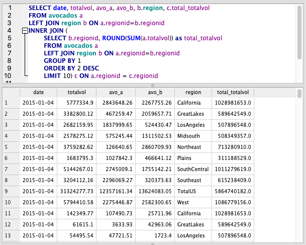

Subqueries can also be used after a FROM or WHERE clause. Let’s illustrate these with a simple example.

FROM Subquery

SELECT AVG(total_totalvol)
FROM (
  SELECT b.regionid, ROUND(SUM(a.totalvol)) as total_totalvol
  FROM avocados a
  LEFT JOIN region b ON a.regionid=b.regionid
  GROUP BY 1
  ORDER BY 2 DESC
  LIMIT 10)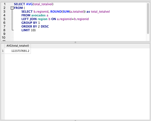

WHERE Subquery

SELECT *
FROM avocados
WHERE regionid IN (
  SELECT regionid
  FROM  region 
  WHERE region LIKE 'West%')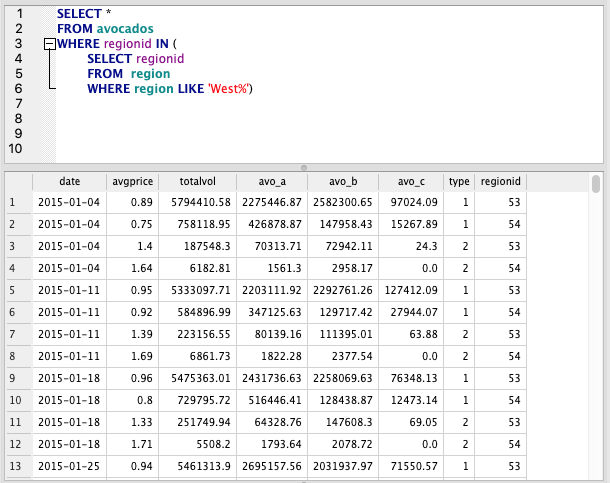

Common Table Expressions

A Common Table Expression (aka CTE, aka WITH statement) is a temporary data set to be used as part of a query. It only exists during the execution of that query; it cannot be used in other queries even within the same session

Common Table Expressions are recommended if you plan to reuse the subquery within the same query because the subquery is temporarily saved to memory, meaning it doesn’t need to be run multiple times. They generally also look much cleaner, so if you are sharing code it can be helpful for legibility.

In this example we’ll just use a CTE in a way that could also be done with a subquery and we’ll take the INNER JOIN example from above.

Here, we specify the subquery above our main query. We name it ‘top’ and specify the column names, then write a subquery. We can now call ‘top’ throughout the query to use this.

If we call it multiple types, SQL only has to generate the table once.

WITH top (regionid, total_totalvol) AS (
SELECT b.regionid, ROUND(SUM(a.totalvol))
  FROM avocados a
  LEFT JOIN region b ON a.regionid=b.regionid
  GROUP BY 1
  ORDER BY 2 DESC
  LIMIT 10)
  
SELECT date, totalvol, avo_a, avo_b, b.region, top.total_totalvol
FROM avocados a
LEFT JOIN region b ON a.regionid=b.regionid
INNER JOIN top ON a.regionid = top.regionid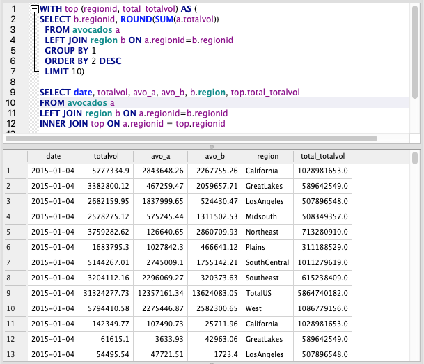

Window Functions

From PostgreSQL’s documentation:

A window function performs a calculation across a set of table rows that are somehow related to the current row. This is comparable to the type of calculation that can be done with an aggregate function. But unlike regular aggregate functions, use of a window function does not cause rows to become grouped into a single output row — the rows retain their separate identities. Behind the scenes, the window function is able to access more than just the current row of the query result.

Basically — we can use Window functions to look at rows above and below each row.

For more information and challenges, take a look at this fantastic resource: https://www.windowfunctions.com/

Running Total

The OVER ORDER BY sequence is the window function. OVER is almost like a GROUP BY, specifying how we want to construct our sum. The ORDER BY allows us to create the running total

SELECT 
   date
 , avo_a
 , SUM(avo_a) OVER (ORDER BY date) AS running_total
FROM avocados
WHERE regionid =1 AND type =1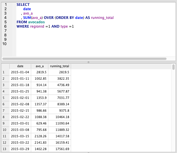

Total by date

Here, we use PARTITION BY to group the SUM by a given column (Date in this case)

SELECT 
   date
 , avo_a
 , type
 , SUM(avo_a) OVER (PARTITION BY date) AS date_total
FROM avocados
WHERE regionid =1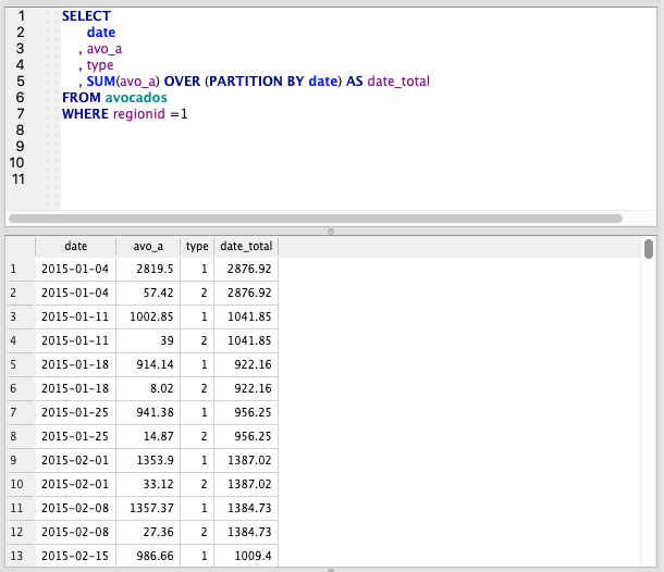

Moving Average

This is where things start to heat up. By using AVG and ORDER BY date, we can specify ROWS to take a moving average. 3 PRECEDING is a 3 day moving average, but we can specify any number.

SELECT 
   date
 , avo_a
 , AVG(avo_a) OVER (ORDER BY date ASC  ROWS 3 PRECEDING) AS date_total
FROM avocados
WHERE regionid =1 AND type=1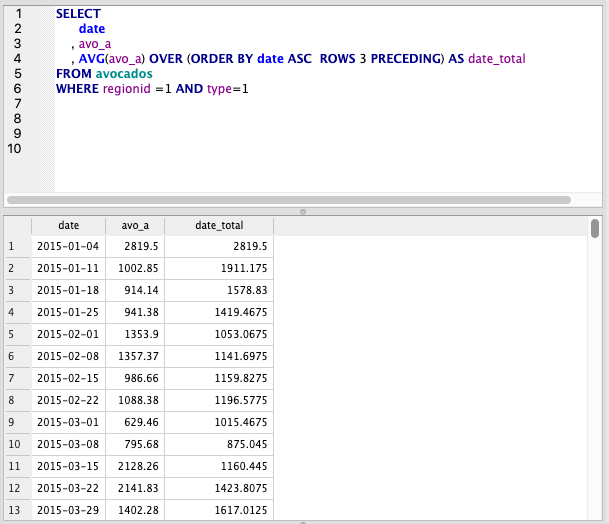

Get First Row

Let’s say we have varying end dates for each region. We can use Window Functions combined with a Subquery to get the first or last dates.

First, let’s define what our Subquery will be. The below query adds a row number, grouped by region id and ordered from most recent to oldest. We can select the first row from each grouping to get the newest date

SELECT 
   date
   , regionid
   , ROW_NUMBER() OVER (PARTITION BY regionid ORDER BY date desc) AS row_number
FROM avocados
ORDER BY regionid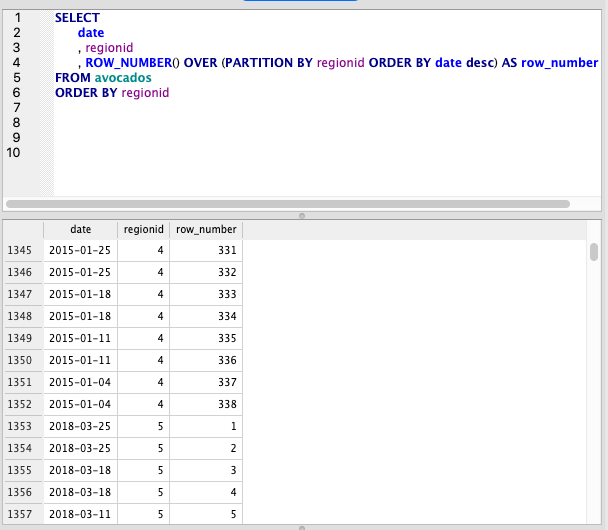

Now, we subquery the original and take only the first row.

SELECT date, regionid
FROM
  (SELECT 
     date
     , regionid
     , ROW_NUMBER() OVER (PARTITION BY regionid 
     ORDER BY date desc) AS row_number
  FROM avocados
  ORDER BY regionid)
WHERE row_number = 1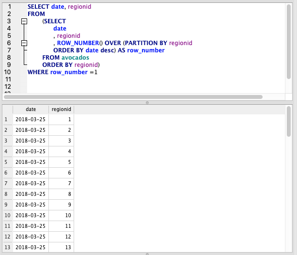

Conclusion

Mastering these is a bonus, many of these functions help to optimise your queries or roll data up. This can be important when working with large datasets as rolling up in the SQL layer of your analysis pipeline will speed things up down the line.

More articles:

Contact me: