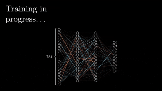
Fit Your LLM on a single GPU with Gradient Checkpointing, LoRA, and Quantization: a deep dive

Whoever has ever tried to fine-tune a Large Language Model knows how hard it is to handle the GPU memory.

“RuntimeError: CUDA error: out of memory”.

This error message has been haunting my nights.

3B, 7B, or even 13B parameters models are large and the fine-tuning is long and tedious. Running out of memory during training can be both frustrating and costly.

But don’t worry, I got you!

In this article, we’re going through 3 techniques you have to know or already use without knowing how they work: Gradient Checkpointing, Low-Rank Adapters, and Quantization.

These will help you avoid running out of memory during your training and save you a lot of time.

If you’re not familiar with fine-tuning an LLM, I wrote an article on this topic where I walk you through fine-tuning Bloom-3B on the Lord Of The Rings books.

Let’s start!

Gradient checkpointing

Gradient checkpointing is a technique that uses dynamic computing to store only a minimal number of layers during neural network training.

To understand this process, we need to understand how back-propagation is performed and how layers are stored in the GPU memory throughout the process.

Forward and backward propagation fundamentals

The forward and backward propagations are the two phases of deep neural network training.

During the forward pass, the input is vectorized (transforming images into pixels and texts into embeddings), and each element is processed throughout the neural network via a succession of linear multiplications and activation functions (non-linear functions such as sigmoid or ReLU).

The output of the neural network, referred to as the head, is designed to produce the desired output, such as classification or next-word prediction. The vectorized prediction is then compared to the expected result, and the loss is calculated using a specific loss function, such as cross-entropy, L2-norm, etc…

The back-propagation can begin.

Based on the loss value, the weights and biases of each layer will be updated with the objective of minimizing the loss. This update process starts from the end of the neural network and propagates toward the beginning.

To dig more into the basics, I suggest you have a look at the 3Blue1Brown videos and this nice article about back-propagation.

Now we give a quick and simple reminder of the neural network training algorithm, let’s talk about how calculations are stored in the memory.

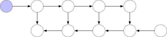
“Poor-memory” algorithm

A simple approach would be to retain only the essential layers required for the back-propagation and release them from memory once their usage is complete.

But as you can observe in the image above, the peak number of layers stored in memory at the same time is non-optimal. We need to find a way to store a lower number of elements in memory while keeping the back-propagation working.

“Poor computation time” algorithm

A way to reduce the memory footprint would consist in re-computing each layer during the back-propagation from the beginning of the neural network.

But in this case, the computation time would increase significantly, making the training unpracticable in the case of large models.

So what if we could have the best of both worlds?

Who said gradient checkpointing?

Optimize computation and memory with Gradient checkpointing

This technique saves “checkpoints” to compute “missing” layers during back-propagation.

In simpler terms, instead of computing the layer from the beginning, as demonstrated in the previous example, the algorithm starts the computation from the nearest checkpoint.

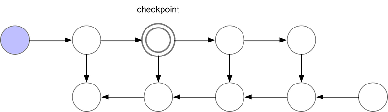
An optimal strategy to balance memory storage and computation time would be to take a checkpoint every O(sqrt(n)), with n the number of layers. This way, the number of additional computations for a backward computation would correspond to one additional feed-forward pass.

This technique enables training larger models on smaller GPUs at the expense of an additional computational time (~20%).

Sources: * Training Deep Nets with Sublinear Memory Cost, Tianqi Chen’s paper

* Fitting larger networks into memory, from Yaroslav Bulatov’s Medium article

How to implement gradient checkpointing with Transformers

You can easily use the gradient checkpointing technique with the following code in the transformerslibrary.

from transformers import AutoModelForCausalLM, TraininArguments

model = AutoModelForCausalLM.from_pretrained(
    model_id,
    use_cache=False, # False if gradient_checkpointing=True
    **default_args
)
model.gradient_checkpointing_enable()

Low-Rank Adapters (LoRA)

LoRA is a technique developed by the Microsoft team to accelerate the fine-tuning of large language models. To evaluate this approach, they implemented it on GPT-3 175B and achieved a substantial reduction in the number of trained parameters.

But how does it work?

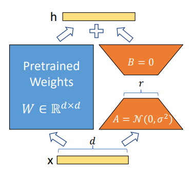
Their approach consists in freezing all parameters of a pretrained model and embedding new trainable parameters to specific modules in the transformers’ architecture, like the Attention modules (query, key, value but also works for others modules).

To implement those adapters, they exploit the linearity of dense layers, shown in the following equation, with x (dimension: d) and h (dim: k) as the layers before and after multiplication, Wo as the pretrained weights, and B & A as the new weights matrices.

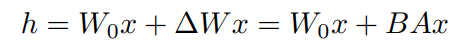
The dimension of the matrices B & A are respectively (d x r) and (r x k) with r << min(d, k).

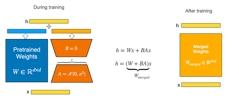
In other words, new dense layers are graffed on the existing ones without complexifying the training process. But instead of training the integrality of parameters, only a tiny portion is updated!

During the fine-tuning process, the weights matrix BA is initialized to 0 and follows a linear scale of α/r, with α a constant. When optimizing the weights with the Adam algorithm, α is roughly the same as the learning rate.

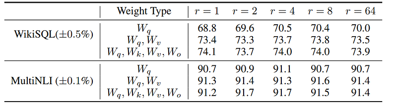
Different LoRA configurations have been tested and it results from the paper that r=8 (or above) applied to a variety of modules performs the best.

Once your LoRA model is fine-tuned, you can merge the weights together to obtain a single model or save only the adapters independently and load the pretrained model separately from the existing ones.

How to implement LoRA in your code?

It is possible to exploit the LoRA technique by using the PEFT library developed by the Hugging Face team.

from peft import LoraConfig, TaskType

lora_config = LoraConfig(
        r=16,
        lora_alpha=16,
        target_modules=["query_key_value"]
        lora_dropout=0.1,
        bias="none",
        task_type=TaskType.CAUSAL_LM,
    )

# OR 
# target_modules = [
#            "query_key_value",
#            "dense",
#            "dense_h_to_4h",
#            "dense_4h_to_h",
#     ]

You can also target all the dense layers in the transformers architecture:

# From https://github.com/artidoro/qlora/blob/main/qlora.py
def find_all_linear_names(args, model):
    cls = torch.nn.Linear
    lora_module_names = set()
    for name, module in model.named_modules():
        if isinstance(module, cls):
            names = name.split('.')
            lora_module_names.add(names[0] if len(names) == 1 else names[-1])

You’ve now just to add the “initialized” adapters to a pretrained model of your choice.

from transformers import AutoModelForCausalLM
from peft import get_peft_model

model = AutoModelForCausalLM.from_pretrained(model_id)
lora_model = get_peft_model(model, peft_config)
lora_model.print_trainable_parameters()

# "trainable params: 1855499 || all params: 355894283 || trainable%: 0.5213624069370061"

Once trained, you can either save the adapters separately or merged them into the model.

# Save only adapaters
lora_model.save_pretrained(...)

# Save merged model
merged_model = lora_model.merge_and_unload()  
merged_model.save_pretrained(...)

Sources: * Low-Rank Adapters paper * Hugging Face PEFT — LoRA documentation

Quantization

I cannot talk about LoRA without talking about quantization. Both of these techniques were fused in the paper QLORA: Efficient Finetuning of Quantized LLMs, and were later implemented into the Hugging Face through the library bitsandbytes , peft , and accelerayte .

Let’s dig into it!

What is the quantization process?

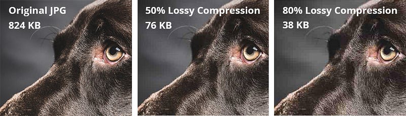
Quantization is a technique that reduces the precision of an element without losing the overall meaning of it.

For instance, in the case of a picture, quantization consists in reducing the number of pixels, while keeping a decent resolution of the image.

But how does it apply to float numbers? Wait a minute, what is a float number?

Certainly, one cannot grasp the concept of quantization without first understanding how computers represent numbers.

Float numbers fundamentals

Our computers are binary, which means they only exchange information through 0 and 1’s.

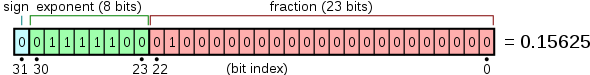
In order to represent numbers, a specific system called the Floating-Point format was designed, which allows computers to understand a wide range of numerical values. The most common representation is the single-precision floating-point format, composed of 32 bits (one bit = 0 or 1).

Various formats exist, such as half-precision (16 bits) or double-precision (64 bits). In short, the greater the number of bits used, the broader the range of numbers that can be accommodated.

Here’s a video I suggest you watch if you want to know how the float-point format works:

Ok great Jérémy, but what do I do with that information?

What if I tell you you can still achieve great performance without this degree of precision?

Models like GPT-3.5 or Bloom-175B are really large (as you may understand since they’re composed of a bunch of parameters.

In FP32 format, this would represent:

175*10⁹. 4 bytes = 700Gb, or 350Gb in half-precision, which would have to be stored in the GPU for the fine-tuning process!

Remember than 1 byte = 8 bits!

So how do we shrink these models?

Quantization: from FP32 to Int8

As you may have understood if you have watched the youtube video above, Int8 represents any number between [-127, 127].

1 bit for the sign, and 7 bit for the number: 2⁷ = 128, And don’t forget 0 ! Thus [-127, 127]

Let’s say you want to reduce a vector of float numbers into Int8 format:

v = [-1.2, 4.5, 5.4, -0.1]

What you can do is define the maximum of v (here 5.4) and scale all the numbers into the range of Int8 [-127, 127]. To do this, you need to calculate the coefficient

α = 127 / max(v) = 127 / 5.4 ~ 23.5

Now if you scale all numbers in v by α, and you round the result, you get:

α.v = [-28, 106, 127, -2]

Now, if you want to de-quantize this vector, you just have to do the opposite maneuver, and you get back to the initial vector!

v = [-1.2, 4.5, 5.4, -0.1] after de-quantization

Great, you performed quantization and de-quantization without losing any information!

At least that’s what you might think, but in reality, we did lose precision when rounding each value. Nevertheless, in this specific case, the difference is not substantial because we decided to represent numbers with only one decimal.

Now, what happens in the case of the presence of an outlier?

Let’s say we now have this vector:

v’ = [-1.2, 70, 5.4, -0.1]

The highest number is now 70, which can be considered an outlier. And if we reproduce the exact same process, we got after qe-quantization:

de-quantized v’ = [-1.1, 70, 5.5, 0.0]

A loss of precision starts to appear!

Now, let’s consider the same loss applied to an LLM consisting of 7 billion parameters: the lack of precision will accumulate across the neural network, causing the complete loss of meaningful information and resulting in pure noise.

Furthermore, let’s remember we chose 8-bit format, but the result would be much worse with 4-bit or even 3-bit. Try it yourself!

The problem is that at a scale of 6.7B parameters and above, 75% of hidden state sequences are affected (with outliers). So this absolutely wrecks quantization, Tim Dettmers

But a group of people found a way to apply quantization to LLMs!

The LLM.int8( ) made quantization possible at large scales

The paper LLM.int8(): 8-bit Matrix Multiplication for Transformers at Scale introduced a method to bypass this outlier issue.

Instead of quantizing the integrality of parameters, which would lead to a decrease in performance as we have just showcased, quantization is used during the matrices multiplication process, combining mixed-precision decomposition and vector-wise quantized (see the image below)

In other words, during the matrices multiplication process, vectors containing outliers (above a threshold) are extracted from the weights matrix resulting in two multiplications. Small numbers matrices (representing 99.9% of the values according to the paper) are quantized, while large numbers are kept in FP16.

The small-numbers-multiplication output is then de-quantized, and added to the other output, following the mixed_precision decomposition principles.

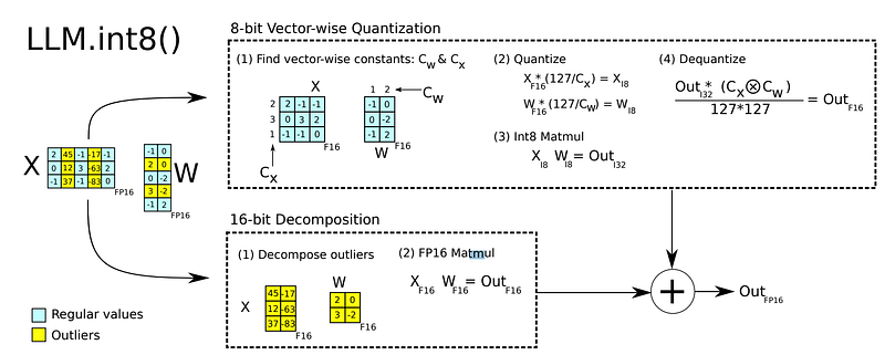
Important notes: The quantization technique introduced here is used during inferences only (matrix multiplications), which means you actually don’t have a lighter model composed of 8-bits numbers! However, the GPU memory footprint during inference is reduced, which is different! You actually even have a slighlty heavier model because of this technique implementation! (by 0.1% for models up to 13B according to the paper)

Experiments on BLOOM-175B showed a reduction of the memory footprint by a factor of 1.96x without any performance degradation!

This technique enables access to large models that could not previously fit into GPU memory. Then Hugging Face spread it worldwide!

Does it mean you can fine-tune this quantized model?

No.

Indeed, recent papers have shown that this technique only works for inferences and is not suitable for training (source). But does it mean we cannot fine-tune a quantized model?…

You probably know where I’m heading with this.

What if we could reduce the GPU memory footprint using quantization, AND train new adapters with the LoRA technique?

QLoRA was born! And the research team succeeded to quantize the pretrained model to 4-bit!

In the paper, new techniques have been implemented to successfully quantize the models, like double-quantization and 4-bit NormalFloat that I haven’t mentioned in this article. If you want to know more about it, I suggest you to read the QLoRA paper, in addition to checking out the blog post from Hugging Face.

How to use quantization in your code?

First, you need to install the bitsandbytes and accelerate libraries

pip install -q bitsandbytes
pip install -q accelerate
pip install -q peft==0.4.1

You can then load the model with the 4-bit or 8-bit quantization by passing the argument load_in_4bit=True or load_in_8bit=Truewhen calling the from_pretrained method .

from transformers import AutoModelForCausalLM
model = AutoModelForCausalLM.from_pretrained("facebook/opt-350m", 
               load_in_4bit=True, 
               device_map="auto"
      )
...

You can also play with the advanced usage with the BitsAndBytesConfig class.

from transformers import BitsAndBytesConfig

nf4_config = BitsAndBytesConfig(
   load_in_4bit=True,
   bnb_4bit_quant_type="nf4",
   bnb_4bit_use_double_quant=True,
   bnb_4bit_compute_dtype=torch.bfloat16
)

model_nf4 = AutoModelForCausalLM.from_pretrained(
                          model_id, 
                          device_map="auto"
                          quantization_config=nf4_config
                          )

Your model is almost ready for inferences.

Indeed, to enable your model to run nicely, you need to:

• Freeze the quantized parameters to prevent any training,
• Cast all layer norms and the LM head in FP32 to ensure the stability of your model (which haven’t been quantized)
• model.enable_input_require_grad() in case you use gradient checkpointing

for name, param in model.named_parameters():
    # freeze base model's layers
    param.requires_grad = False

# cast all non int8 or int4 parameters to fp32
for param in model.parameters():
  if (param.dtype == torch.float16) or (param.dtype == torch.bfloat16):
      param.data = param.data.to(torch.float32)

if use_gradient_checkpointing:
    # For backward compatibility
    model.enable_input_require_grads()

This preparation is now handled in the latest peft==0.4.1 library with the prepare_model_for_kbit_training() method (source code).

That’s it! You now have a quantized model!

Source: * A Gentle Introduction to 8-bit Matrix Multiplication for transformers at scale, Hugging Face blog post * LLM.int8(): 8-bit Matrix Multiplication for Transformers at Scale, paper * QLORA: Efficient Finetuning of Quantized LLMs, paper * Floating point numbers, youtube * Tim Dettmers blog post about LLM.int8() * Making LLMs even more accessible with bitsandbytes, 4-bit quantization and QLoRA, Hugging Face blog post

Let’s wrap up in one code!

Now you have an overview of Gradient Checkpointing, LoRA, and Quantization, let’s write the code to prepare an LLM from the Hugging Face hub for fine-tuning.

pip install -q -U bitsandbytes
pip install -q -U git+https://github.com/huggingface/transformers.git
pip install -q -U git+https://github.com/huggingface/peft.git
pip install -q -U git+https://github.com/huggingface/accelerate.git

from transformers import (
        AutoModelForCausalLM,
        BitsAndBytesConfig
)
from peft import (
        get_peft_model,
        LoraConfig,
        TaskType,
        prepare_model_for_kbit_training
)

# Import the model
gradient_checkpointing = True
model = AutoModelForCausalLM.from_pretrained(
        args.model_id,
        use_cache=False if gradient_checkpointing else True,  # this is needed for gradient checkpointing
        device_map="auto",
        load_in_4bit=True
    )

# Prepare the model (freeze, cast FP32, enable_require_grads, activate gradient checkpointing)
model = prepare_model_for_kbit_training(
                    model, 
                    use_gradient_checkpointing=gradient_checkpointing
    )

# Prepare Peft model by adding Lora
peft_config = LoraConfig(
        r=64,
        lora_alpha=16,
        target_modules=modules,
        lora_dropout=0.1,
        bias="none",
        task_type=TaskType.CAUSAL_LM,
    )

model = get_peft_model(model, peft_config)

Your model is now ready to be fine-tuned with optimal GPU memory management!

Side note

Hugging Face has made the process much easier by creating SFTTrainer, a subclass of Trainer that handles everything we have talked about until now.

In a few lines of code, you can prepare your model for efficient fine-tuning with quantization and Lora.

I suggest you have a look at the official documentation.

from trl import SFTTrainer

model = AutoModelForCausalLM.from_pretrained(
    "EleutherAI/gpt-neo-125m",
    load_in_4bit=True,
    device_map="auto",
)

trainer = SFTTrainer(
    model,
    train_dataset=dataset,
    dataset_text_field="text",
    torch_dtype=torch.bfloat16,
    peft_config=peft_config,
)

trainer.train()

To conclude

In this article, we addressed a challenge that arises during the fine-tuning of Large Language Models: how to fit the training on a single GPU.

We focused on 3 techniques to reduce the memory footprint: gradient checkpointing, LoRA, and Quantization (which lead us to QLoRA).

We then saw how to apply these techniques to our code by leveraging the Hugging Face implementations with PEFT, BitsAndBytes, and Transformers.

The goal of this article was to provide a deep, yet simple, view of the existing techniques you can leverage to fine-tune your own LLMs in your projects.

I’m convinced that using a technique already implemented in libraries is a thing, but knowing what it does and when to use it will make you a better ML Engineer / Data Scientist!

I hope you enjoyed the reading!

I didn’t think I would dig so deep into papers and code repositories to write this article. But overall it was worth it since I learned so much in the process!

You can join my newsletter to get notified of my latest articles.

If you enjoy reading stories like these and want to support me as a writer, you can do it by getting a Medium subscription (it’s $5 a month, giving you unlimited access to articles like this one, and I get a small commission without any additional fee for you!).

Happy coding!