
Feature Importance Using XGBoost (Python Code Included)

A few months ago I wrote an article discussing the mechanism how people would use XGBoost to find feature importance. Since then some reader asked me if there is any code I could share with for a concrete example.
And here it is. In this piece, I am going to explain how to generate feature importance plots from XGBoost using tree-based importance, permutation importance as well as SHAP.
Data and Packages
I am going to use the dataset of NYC flights arrival delay in 2013 (from rdatasets), and build data to predict that variable.
Packages that are needed include:
- pandas
- statsmodels
- matplotlib
- numpy
- scikit-learn
- shap
- category_encoders
- XGBoost
import statsmodels.api as sm
import pandas as pd
import matplotlib.pyplot as plt
import numpy as np
from sklearn.metrics import mean_squared_error
from sklearn.model_selection import train_test_split
from sklearn.inspection import permutation_importance
import shap
import category_encoders as ce
import xgboost as xgb
df = sm.datasets.get_rdataset('flights', 'nycflights13').data
df.info()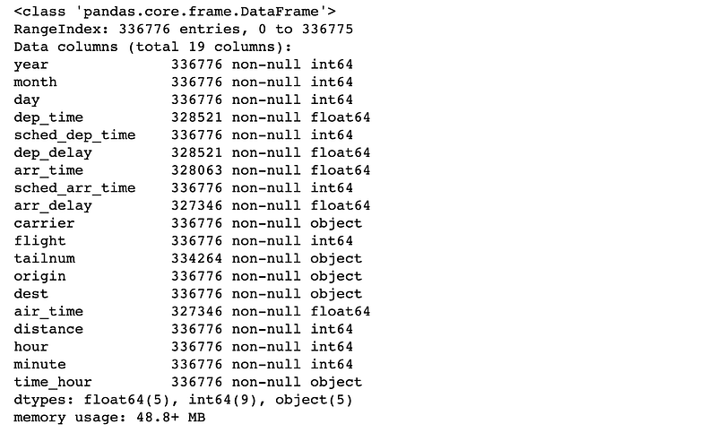
We would need to check how many are null:
df.isnull().sum()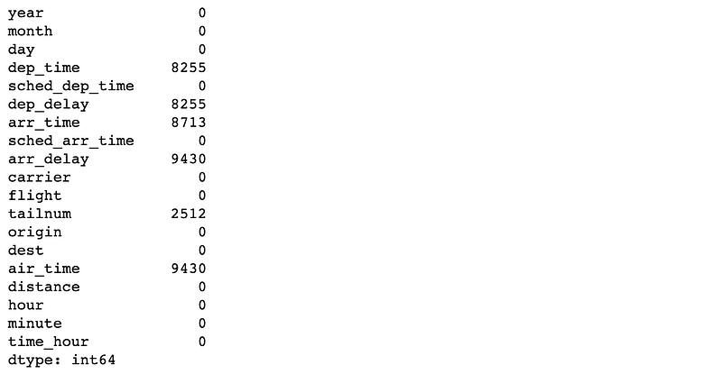
As this model will predict arrival delay, the Null values are caused by flights did were cancelled or diverted. These can be excluded from this analysis.
df.dropna(inplace=True)df['arr_hour'] = df.arr_time.apply(lambda x: int(np.floor(x/100)))
df['arr_minute'] = df.arr_time.apply(lambda x: int(x - np.floor(x/100)*100))
df['sched_arr_hour'] = df.sched_arr_time.apply(lambda x: int(np.floor(x/100)))
df['sched_arr_minute'] = df.sched_arr_time.apply(lambda x: int(x - np.floor(x/100)*100))
df['sched_dep_hour'] = df.sched_dep_time.apply(lambda x: int(np.floor(x/100)))
df['sched_dep_minute'] = df.sched_dep_time.apply(lambda x: int(x - np.floor(x/100)*100))
df.rename(columns={'hour': 'dep_hour','minute': 'dep_minute'}, inplace=True)We know the column we are going to predict is ‘arr_delay’, so we will use the rest columns as features to predict that.
We also use a leave-one-out encoder as it creates a single column for each categorical variable instead of creating a column for each level of the categorical variable like one-hot-encoding. This makes interpreting the impact of categorical variables with feature impact easier.
target = 'arr_delay'
y = df[target]
X = df.drop(columns=[target, 'flight', 'tailnum', 'time_hour', 'year', 'dep_time', 'sched_dep_time', 'arr_time', 'sched_arr_time', 'dep_delay'])
X_train, X_test, y_train, y_test = train_test_split(X, y, test_size=0.3, random_state=1)encoder = ce.LeaveOneOutEncoder(return_df=True)
X_train_New = encoder.fit_transform(X_train, y_train)
X_test_New = encoder.transform(X_test)Now we will use XGBoost to build the model, and do the fit.
model = xgb.XGBRegressor(n_estimators=500, max_depth=5, eta=0.05)
model.fit(X_train_New, y_train)
rmse = np.sqrt(mean_squared_error(y_test, model.predict(np.ascontiguousarray(X_test_New))))rmse42.92687222323455
We can see the RMSE is 42.92.
Let’s check the feature importance now. Below is the code to show how to plot the tree-based importance:
feature_importance = model.feature_importances_
sorted_idx = np.argsort(feature_importance)
fig = plt.figure(figsize=(12, 6))
plt.barh(range(len(sorted_idx)), feature_importance[sorted_idx], align='center')
plt.yticks(range(len(sorted_idx)), np.array(X_test.columns)[sorted_idx])plt.title('Feature Importance')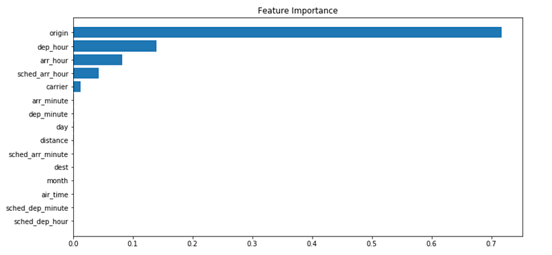
We can also see the Permutation Importance:
perm_importance = permutation_importance(model, np.ascontiguousarray(X_test_New), y_test, n_repeats=10, random_state=1066)
sorted_idx = perm_importance.importances_mean.argsort()
fig = plt.figure(figsize=(12, 6))
plt.barh(range(len(sorted_idx)), perm_importance.importances_mean[sorted_idx], align='center')
plt.yticks(range(len(sorted_idx)), np.array(X_test.columns)[sorted_idx])
plt.title('Permutation Importance')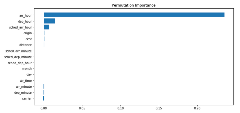
Then we can check the SHAP values and plot the mean absolute values:
explainer = shap.Explainer(model)
shap_values = explainer(np.ascontiguousarray(X_test_New))
shap_importance = shap_values.abs.mean(0).values
sorted_idx = shap_importance.argsort()
fig = plt.figure(figsize=(12, 6))
plt.barh(range(len(sorted_idx)), shap_importance[sorted_idx], align='center')
plt.yticks(range(len(sorted_idx)), np.array(X_test.columns)[sorted_idx])
plt.title('SHAP Importance')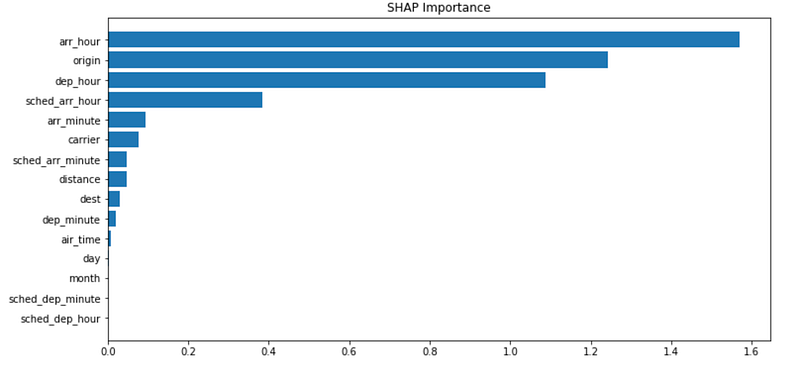
In fact, SHAP contains a function to plot this directly.
shap.plots.bar(shap_values, max_display=X_test_loo.shape[0])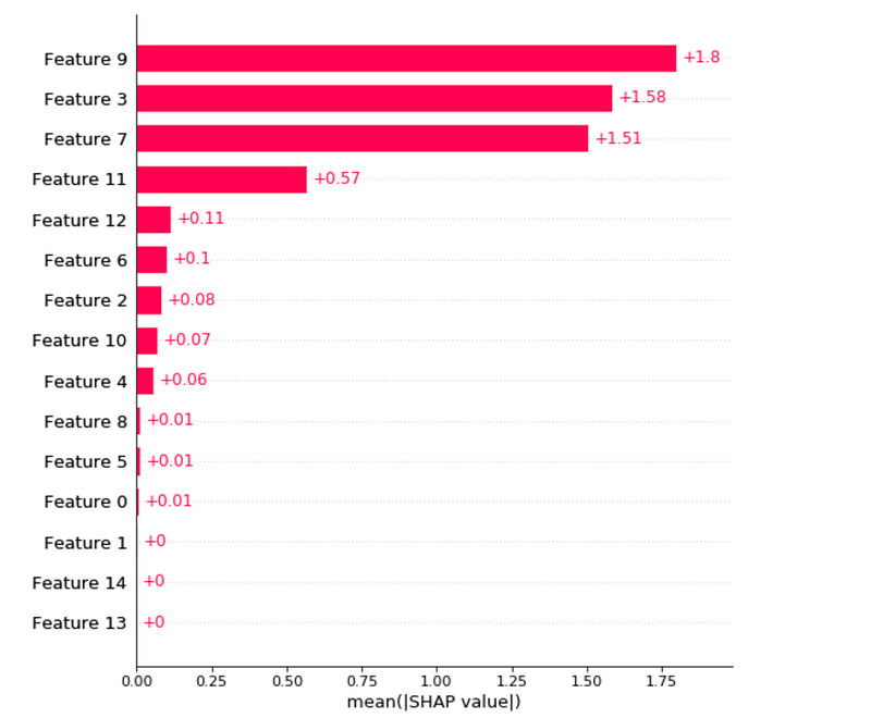
This clearly tells the importance across all the features!
Thanks for Reading!
If you enjoyed it, please follow me on Medium for more. It’s great cardio for your 👏 AND will help other people see the story.
If you want to continue getting this type of article, you can support me by becoming a Medium subscriber.


