Face Recognition Example
Scikit-learn tutorial
I have over forty years of experience writing software including applications written in C/C++. Java, Pascal, Fortran, and various microprocessor assembly languages, just to name a few.
This story is about the scikit-learn application example of face recognition.
This ski kit-learn guide aims to illustrate some of the main features that scikit-learn provides. It assumes a very basic working knowledge of machine-learning practices (model fitting, predicting, cross-validation,
In a previous story, I walked through a ski kit-learn example of cross-validation.
``Scikit-learn`` is an open-source machine learning library that supports supervised and unsupervised learning. It also provides various tools for model fitting, data preprocessing, model selection, model evaluation, and many other utilities.
The examples are written in the python programming language code. I will try to annotate the program explaining what is happening.
Below is the scikit-learn example application of face recognition. My annotations will be in bold italic.
“”” Beginning of block comment.
===================================================
Faces recognition example using eigenfaces and SVMs
===================================================
The dataset used in this example is a preprocessed excerpt of the
“Labeled Faces in the Wild”, aka LFW_:
http://vis-www.cs.umass.edu/lfw/lfw-funneled.tgz (233MB)
.. _LFW: http://vis-www.cs.umass.edu/lfw/
“”” Ending of the block comment.
# %% The # starts a comment the % is the start of the specifier or modulus. #Three double-quotes start a comment block and three more double quotes #end the comment block.
from time import time # Import functions from library modules.
import matplotlib.pyplot as plt # scikit-learn plotting function.
from sklearn.model_selection import train_test_split # dataset splitting # # #function into train and test parts.
from sklearn.model_selection import RandomizedSearchCV #cross #validation
from sklearn.datasets import fetch_lfw_people # Dataset explained above in #block comment.
from sklearn.metrics import classification_report
‘’’’’’
A Classification report is used to measure the quality of predictions from a classification algorithm. How many predictions are True and how many are False. More specifically, True Positives, False Positives, True Negatives, and False Negatives are used to predict the metrics of a classification report
‘’’’
from sklearn.metrics import ConfusionMatrixDisplay # Compute confusion #matrix to evaluate the accuracy of classification.
from sklearn.preprocessing import StandardScaler # In Machine Learning, #StandardScaler is used to resize the distribution of values so that the #mean of the observed values is 0 and the standard deviation is 1.
from sklearn.decomposition import PCA # PCA using python
from sklearn.svm import SVC # sklearn.svm.svc
from sklearn.utils.fixes import loguniform # The loguniform distribution ###(also called the reciprocal distribution) is a two-parameter distribution.
# %%
# Download the data, if not already on disk, and load it as numpy arrays
‘’’’’’
A numpy array is a grid of values, all of the same type, and is indexed by a tuple of nonnegative integers. The number of dimensions is the rank of the array; the shape of an array is a tuple of integers giving the size of the array along each dimension. numpy is a component of scikit-learn
fetch_lfw_people down downloads the data if not a; ready on disk.
“””
lfw_people = fetch_lfw_people(min_faces_per_person=70, resize=0.4)
# introspect the images arrays to find the shapes (for plotting)
n_samples, h, w = lfw_people.images.shape
# for machine learning we use the 2 data directly (as relative pixel
# positions info is ignored by this model)
X = lfw_people.data
n_features = X.shape[1]
# the label to predict is the id of the person
y = lfw_people.target
target_names = lfw_people.target_names
n_classes = target_names.shape[0]
print(“Total dataset size:”)
print(“n_samples: %d” % n_samples)
print(“n_features: %d” % n_features)
print(“n_classes: %d” % n_classes)
# %%
# Split into a training set and a test and keep 25% of the data for testing. #split the data.
X_train, X_test, y_train, y_test = train_test_split(
X, y, test_size=0.25, random_state=42
)
scaler = StandardScaler()
X_train = scaler.fit_transform(X_train)
X_test = scaler.transform(X_test)
# %%
# Compute a PCA (eigenfaces) on the face dataset (treated as unlabeled
# dataset): unsupervised feature extraction / dimensionality reduction
n_components = 150
print(
“Extracting the top %d eigenfaces from %d faces” % (n_components, X_train.shape[0])
)
t0 = time()
pca = PCA(n_components=n_components, svd_solver=”randomized”, whiten=True).fit(X_train)
print(“done in %0.3fs” % (time() — t0))
“””
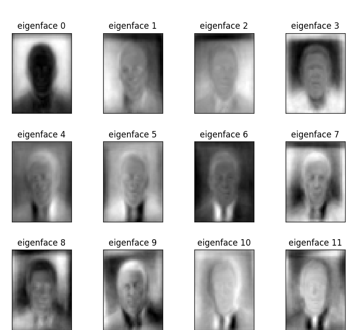
An eigenface (/ˈaɪɡənˌfeɪs/) is the name given to a set of eigenvectors when used in the computer vision problem of human face recognition. The approach of using eigenfaces for recognition was developed by Sirovich and Kirby and used by Matthew Turk and Alex Pentland in face classification.
Eigenvalues are the special set of scalar values that are associated with the set of linear equations most probably in the matrix equations. The eigenvectors are also termed characteristic roots. It is a non-zero vector that can be changed at most by its scalar factor after the application of linear transformations.
“””
eigenfaces = pca.components_.reshape((n_components, h, w))
print(“Projecting the input data on the eigenfaces orthonormal basis”)
t0 = time()
X_train_pca = pca.transform(X_train)
X_test_pca = pca.transform(X_test)
print(“done in %0.3fs” % (time() — t0))
# %%
# Train a SVM classification model
print(“Fitting the classifier to the training set”)
t0 = time()
param_grid = {
“C”: loguniform(1e3, 1e5),
“gamma”: loguniform(1e-4, 1e-1),
}
clf = RandomizedSearchCV(
SVC(kernel=”rbf”, class_weight=”balanced”), param_grid, n_iter=10
)
clf = clf.fit(X_train_pca, y_train)
print(“done in %0.3fs” % (time() — t0))
print(“Best estimator found by grid search:”)
print(clf.best_estimator_)
# %%
# Quantitative evaluation of the model quality on the test set
print(“Predicting people’s names on the test set”)
t0 = time()
y_pred = clf.predict(X_test_pca)
print(“done in %0.3fs” % (time() — t0)) # print the time the #program took.
print(classification_report(y_test, y_pred, target_names=target_names))
ConfusionMatrixDisplay.from_estimator(
clf, X_test_pca, y_test, display_labels=target_names, xticks_rotation=”vertical”
)
plt.tight_layout()
plt.show()
# %%
# Qualitative evaluation of the predictions using matplotlib
def plot_gallery(images, titles, h, w, n_row=3, n_col=4):
“””Helper function to plot a gallery of portraits”””
plt.figure(figsize=(1.8 * n_col, 2.4 * n_row)) # plot figures.
plt.subplots_adjust(bottom=0, left=0.01, right=0.99, top=0.90, hspace=0.35)
for i in range(n_row * n_col):
plt.subplot(n_row, n_col, i + 1)
plt.imshow(images[i].reshape((h, w)), cmap=plt.cm.gray)
plt.title(titles[i], size=12)
plt.xticks(())
plt.yticks(())
# %%
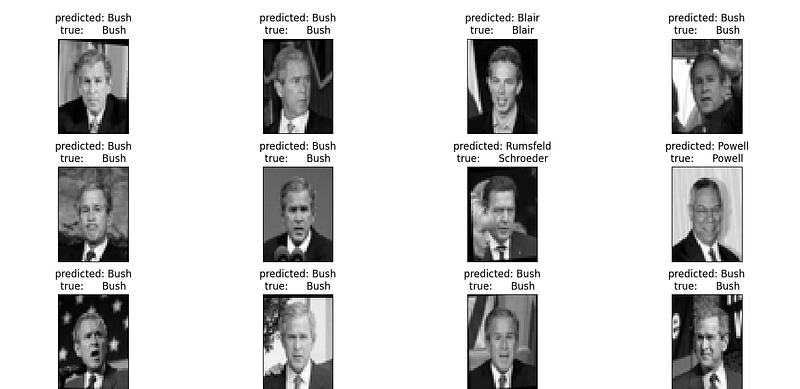
# plot the result of the prediction on a portion of the test set
def title(y_pred, y_test, target_names, i):
pred_name = target_names[y_pred[i]].rsplit(“ “, 1)[-1]
true_name = target_names[y_test[i]].rsplit(“ “, 1)[-1]
return “predicted: %s\ntrue: %s” % (pred_name, true_name)
prediction_titles = [
title(y_pred, y_test, target_names, i) for i in range(y_pred.shape[0])
]
plot_gallery(X_test, prediction_titles, h, w)
# %%
# plot the gallery of the most significative eigenfaces
eigenface_titles = [“eigenface %d” % i for i in range(eigenfaces.shape[0])]
plot_gallery(eigenfaces, eigenface_titles, h, w)
plt.show()
# %%
# Face recognition problem would be much more effectively solved by training
# convolutional neural networks but this family of models is outside of the scope of
# the scikit-learn library. Interested readers should instead try to use pytorch or
# tensorflow to implement such models.
The program output.
[bob@localhost applications]$ python3 plot_face_recognition.py
=================================================== Faces recognition example using eigenfaces and SVMs ===================================================
The dataset used in this example is a preprocessed excerpt of the “Labeled Faces in the Wild”, aka LFW_:
http://vis-www.cs.umass.edu/lfw/lfw-funneled.tgz (233MB)
.. _LFW: http://vis-www.cs.umass.edu/lfw/
Expected results for the top 5 most represented people in the dataset:
================== ============ ======= ========== ======= precision recall f1-score support ================== ============ ======= ========== ======= Ariel Sharon 0.67 0.92 0.77 13 Colin Powell 0.75 0.78 0.76 60 Donald Rumsfeld 0.78 0.67 0.72 27 George W Bush 0.86 0.86 0.86 146 Gerhard Schroeder 0.76 0.76 0.76 25 Hugo Chavez 0.67 0.67 0.67 15 Tony Blair 0.81 0.69 0.75 36
avg / total 0.80 0.80 0.80 322 ================== ============ ======= ========== =======
Total dataset size: n_samples: 1288 n_features: 1850 n_classes: 7 Extracting the top 150 eigenfaces from 966 faces done in 0.453s Projecting the input data on the eigenfaces orthonormal basis done in 0.020s Fitting the classifier to the training set done in 20.822s Best estimator found by grid search: SVC(C=1000.0, class_weight=’balanced’, gamma=0.005) Predicting people’s names on the test set done in 0.064s precision recall f1-score support
Ariel Sharon 1.00 0.69 0.82 13 Colin Powell 0.85 0.78 0.82 60 Donald Rumsfeld 0.67 0.52 0.58 27 George W Bush 0.78 0.95 0.86 146 Gerhard Schroeder 0.75 0.60 0.67 25 Hugo Chavez 0.80 0.27 0.40 15 Tony Blair 0.65 0.61 0.63 36
accuracy 0.78 322 macro avg 0.79 0.63 0.68 322 weighted avg 0.78 0.78 0.76 322
[[ 9 0 0 4 0 0 0] [ 0 47 4 9 0 0 0] [ 0 2 14 9 0 0 2] [ 0 0 1 139 0 0 6] [ 0 0 1 6 15 1 2] [ 0 2 0 4 3 4 2] [ 0 4 1 7 2 0 22]] Warning: Ignoring XDG_SESSION_TYPE=wayland on Gnome. Use QT_QPA_PLATFORM=wayland to run on Wayland anyway. [bob@localhost applications]$
# The warning is just saying gnome on Linux uses different graphics #than x #windows.