XGBoost 2.0: Major update on Tree-based methods

Let’s get a few things out of the equation: DL-based methods are still far inferior to XGBoost when handling tabular data. XGBoost is the most famous algorithm to handle different types of tabular data. There are other versions out there, like LightGBM and others, but they all have very similar architecture except for a few changes here and there. With a new major release, XGBoost 2.0, we’ve got some pretty exciting updates that were due for a long time. So, without wasting any time, let’s dive into the complete history, mechanics, and new updates of XGBoost.

Topics covered in this blog:

• Background
• Decision Trees (heuristic, overfitting, etc)
• Random Forest
• Gradient Boosted Decision Trees
• XGBoost
• What’s new in XGBoost 2.0?

Given that it’s a pretty big article, I would still suggest reading it, at least from Gradient Boosted Decision Trees.

Background

Tree-based methods like Decision Trees, Random Forests, and by extension, XGBoost, excel at handling tabular data for a multitude of reasons. First, their hierarchical structure is inherently adept at modeling the layered relationships often found in tabular formats.

Second, they are particularly effective at automatically detecting and incorporating complex, non-linear interactions between features.

Third, these algorithms are robust to the scale of input features, allowing them to perform well on raw datasets without the need for normalization.

Additionally, they offer the advantage of handling categorical variables natively, bypassing the need for preprocessing techniques like one-hot encoding, although it’s worth noting that XGBoost usually requires numerical encoding.

Finally, the ease with which tree-based models can be visualized and interpreted lends further appeal, especially when making sense of tabular data structures. By leveraging these inherent strengths, tree-based methods — especially advanced ones like XGBoost — are exceptionally well-suited for tackling a broad spectrum of challenges in data science, particularly when dealing with tabular data.

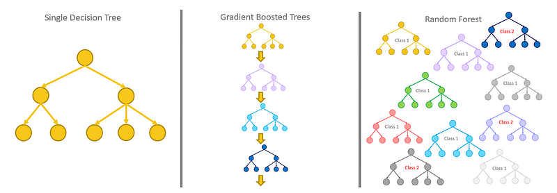
Decision Trees

In a more rigorous mathematical language, a Decision Tree represents a function T:X→Y, where X is the feature space and Y can either be a continuous value (in case of regression) or a class label (in case of classification). We can denote the data distribution as D and the true function f:X→Y. The Decision Tree aims to find T(x) such that it approximates f(x) closely, ideally over a probability distribution D.

Risk and Loss Function

The risk R associated with a tree T, relative to f, is expressed as the expected value of a loss function between T(x) and f(x):

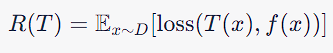
The primary goal of constructing a decision tree is to build a model that generalizes well to new, unseen data. In a perfect world, we would know the true distribution D of the data, and we could directly compute the risk or expected loss for any candidate decision tree. However, in practice, the true distribution is unknown.

Hence, we rely on a subset of available data to make our decisions. This is where the notion of a heuristic method enters the picture.

Heuristic method

A heuristic is a rule of thumb or a practical approach not guaranteed to be perfect or optimal but good enough for immediate goals. In the context of decision trees, heuristic methods like the Gini Index or Information Gain are used to decide how to split a node. The word “heuristic” is important here because these methods do not guarantee the most generalized or least risky tree; they aim for “good enough” solutions based on our sample data.

Gini Index The Gini Index is an impurity measure that quantifies how mixed the classes are in a given node. The formula for the Gini index G for a given node t is:

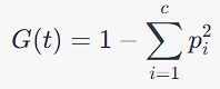
Where p_i is the proportion of samples belonging to class i in node t, and c is the number of classes.

The Gini Index ranges from 0 to 0.5, where a lower value means the node is purer (i.e., contains samples predominantly from one class).

Why Gini Index or Information Gain? Both Gini Index and Information Gain are measures that quantify the “usefulness” of a feature for discriminating between classes. Essentially, they provide a way to evaluate how well a feature separates the data into classes. By selecting the feature that achieves the greatest reduction in impurity (lowest Gini Index or highest Information Gain), you are making a heuristic decision that this is the best local choice for this step in growing the tree.

Overfitting and pruning

Decison trees are notorious for overfitting, especially when they are deep, capturing noise in the data. There are two main strategies to combat this:

1. Cautious Splitting: As the tree grows, continuously monitor its performance on a validation dataset. If performance starts to degrade, this is a signal to stop growing the tree.

2. Post-pruning: Prune nodes that do not provide much predictive power after the tree is fully grown. This is typically done by removing a node and checking if it decreases the validation accuracy. If not, then the node is pruned.

We can’t find an optimally risk-minimized tree because we don’t know the true data distribution D. We instead use heuristic methods like Gini Index or Information Gain to locally optimize the tree based on available data, while techniques like cautious splitting and pruning help to manage the complexity of the model and avoid overfitting.

If you want a full, detailed explanation of Decision Trees:

Random Forests

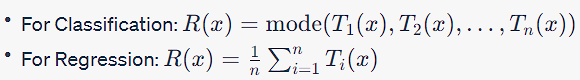
A Random Forest is an ensemble of Decision Trees T_1, T_2, …., T_n where each Decision Tree T_i:X→Y maps an input feature space X to an output Y, which can either be a continuous value (regression) or a class label (classification).

Ensemble Function

The Random Forest ensemble defines a new function R:X→Y which takes a majority vote (classification) or an average (regression) of all the individual tree outputs, mathematically expressed as:

### Data Distribution, True Function, and Heuristic Methods

Like Decision Trees, Random Forests also aim to approximate a true function f:X→Y ideally over a probability distribution D. However, D is typically unknown in practice, making it necessary to use heuristic methods for constructing individual trees.

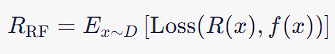
The risk R_RF associated with a Random Forest relative to f is the expected value of a loss function between R(x) and f(x). Given that R is an ensemble of T, the risk is often lower than the risk associated with individual trees, which aids in generalization:

Overfitting and Bagging

Random Forests are less prone to overfitting compared to a single Decision Tree, thanks to bagging and feature randomization, which create diversity among the trees. The risk is averaged out over multiple trees, making the model more resilient to noise in the data.

Bagging in Random Forests achieves multiple objectives: it reduces overfitting by averaging predictions across diverse trees, each trained on a different bootstrap sample, there by making the model more resilient to noise and fluctuations in the data. This also reduces variance, leading to more stable and accurate predictions. The ensemble of trees, capturing different facets of the data, improves the model’s generalization to unseen data. Furthermore, the aggregate of these trees provides robustness, as correct predictions from others often cancel out errors from individual trees. Lastly, the technique can enhance the representation of minority classes in imbalanced datasets, making the ensemble better suited for such challenges.

Heuristic Methods in Random Forest

Heuristic methods like Gini Index or Information Gain are used in constructing individual trees within the Random Forest. However, because each tree is trained on a bootstrap sample and uses a random subset of features, the heuristics are applied in a more diverse setting compared to a single tree, thereby increasing the chance of capturing the underlying data distribution more faithfully.

In summary, a Random Forest is an ensemble model aiming to approximate the unknown true function f and probability distribution D. It employs heuristic methods at the individual tree level but mitigates some limitations through ensemble learning, thus offering a balance between fit and generalization. Techniques like bagging and feature randomization further help reduce the risk and increase the model’s robustness.

Gradient Boosted Decision Trees

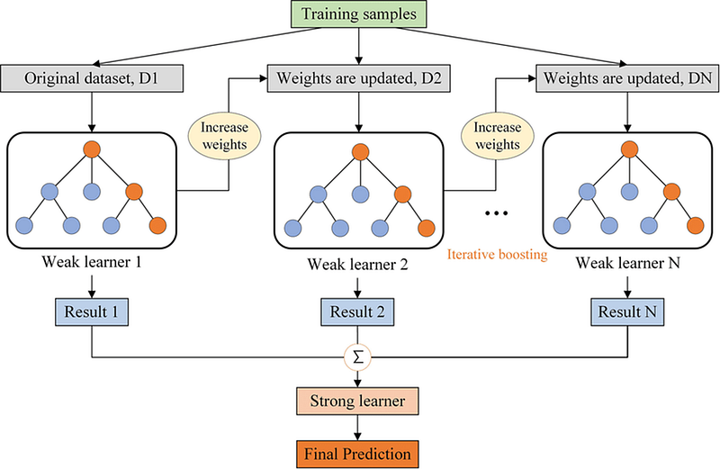
Gradient Boosted Decision Trees (GBDT) is an ensemble method that constructs a strong predictive model by iteratively adding decision trees, with each new tree aiming to correct the mistakes of the existing ensemble. Mathematically, GBDT also represents a function T:X→Y, but instead of finding a single T(x), it forms a sequence of weak learners t_1(x), t_2(x),… that work collectively to approximate the true function f(x). Unlike Random Forest, which builds trees independently through bagging, GBDT builds trees in a sequence, using gradient descent to minimize the difference between the predicted and true values, often expressed through a loss function.

In GBDT, after each tree is built and predictions are made, the residuals (or errors) between the predicted and actual values are computed. These residuals are essentially a form of gradient — indicating how the loss function is changing with respect to its parameters. A new tree is then fit to these residuals, not the original outcome variable, effectively taking a “step” to minimize the loss function using the gradient information. This process is repeated, iteratively refining the model.

So, the term “gradient” signifies the use of gradient descent optimization to guide the sequential building of trees, aiming to continually minimize a loss function and thereby make the model more predictive.

Why is it better than Decision Trees and Random Forest?

1. Reduced Overfitting: Like Random Forest, GBDT also avoids overfitting, but it does so by building shallow trees (weak learners) and optimizing a loss function, rather than by averaging or voting.

2. Boosting Efficiency: GBDT focuses on instances that are hard to classify, adapting more to the problematic areas of the dataset. This can make it more efficient in terms of classification performance compared to Random Forest, which treats all instances equally.

3. Optimized Loss Function: Unlike heuristic methods such as Gini Index or Information Gain, the loss function in GBDT is optimized during training, allowing for a more precise fit to the data.

4. Better Performance: GBDT often outperforms Random Forest when the correct hyperparameters are chosen, particularly in cases where a very accurate model is needed and computational cost is not a primary concern.

5. Flexibility: GBDT can be used for both classification and regression tasks, and it’s easier to optimize because you’re directly minimizing a loss function.

Problems solved

• High Bias in Individual Trees: GBDT can achieve higher performance than individual trees by correcting their errors iteratively.
• Model Complexity: While Random Forest aims to reduce model variance, GBDT offers a fine balance between bias and variance, often achieving better overall performance.

In summary, gradient-boosted decision Trees offer performance, adaptability, and optimization advantages over Decision Trees and Random Forest. They are particularly useful when you require high predictive accuracy and are willing to spend the computational resources to fine-tune the model.

XGBoost

In discussions about tree-based ensemble methods, the spotlight often lands on the standard advantages: robustness to outliers, ease of interpretation, and so forth. However, XGBoost has additional characteristics that set it apart and give it the edge in many scenarios.

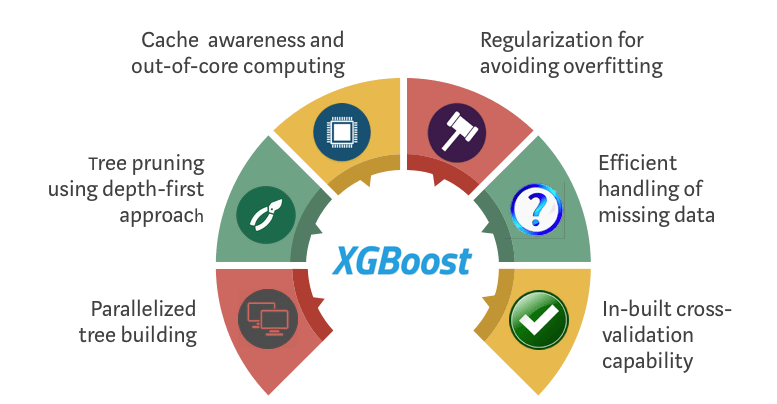
Computational efficiency

Typically, discussions around XGBoost focus on its predictive prowess. Less often highlighted is its computational efficiency, especially when it comes to parallel and distributed computing. The algorithm utilizes features and data points to parallelize the tree construction, enabling it to handle larger datasets and run faster than traditional implementations.

Handling missing data

XGBoost incorporates a unique approach to dealing with missing values. Unlike other models, which usually require a separate preprocessing step, XGBoost can handle missing data internally. During training, the algorithm finds the best imputation value (or direction to move in the tree structure) for missing values, which are then stored for future predictions. This implies that XGBoost’s approach to missing data is adaptive and can vary from node to node, providing a more nuanced handling of such values.

Regularization

While boosting algorithms are inherently prone to overfitting, especially with noisy data, XGBoost directly incorporates L1 (Lasso) and L2 (Ridge) regularization into its objective function during training. This approach provides an additional mechanism to constrain the complexity of individual trees, beyond simply limiting their depth, thereby improving generalization.

Sparsity awareness

XGBoost is designed to work efficiently with sparse data, not just dense matrices. In domains like Natural Language Processing, where bag-of-words or TF-IDF representations are used, the sparsity of the feature matrix can be a significant computational challenge. XGBoost utilizes a compressed memory-efficient data structure, and its algorithm is designed to traverse sparse matrices efficiently.

Customizations

XGBoost allows for immense customization. Beyond the standard hyperparameters like learning rate and tree depth, XGBoost allows users to define custom objective functions and evaluation criteria. This enables it to be adapted to solve very specialized problems that are impossible to solve with a generic implementation.

Hardware optimizations

While less frequently discussed, hardware optimization is an area where XGBoost shines. It is optimized for both memory efficiency and computational speed on the CPU, and it has support for training models on GPU, further accelerating the training process.

Feature importance and model Interpretability

Most ensemble methods offer feature importance metrics, including Random Forest and standard Gradient Boosting. However, XGBoost provides a more comprehensive suite of feature importance measures, including Gain, Frequency, and Coverage, allowing for a more detailed interpretability of the model. This can be critical when you need to understand what features are important and how they contribute to predictions, a nuance often lost in standard metrics.

Early Stopping

Another under-discussed feature is early stopping. While techniques like cautious splitting and pruning are employed to combat overfitting, XGBoost provides a more automated approach. The training process can be halted as soon as the model’s performance stops improving on a held-out validation dataset, thereby saving computational resources and time.

Native handling of Categorical variables

While I mentioned that tree-based algorithms handle categorical variables well, it’s worth noting that XGBoost takes a unique approach. Instead of requiring one-hot or ordinal encoding, you can leave categorical variables as they are. XGBoost handles categorical variables more nuanced than a simple binary split and can capture complex relationships without additional preprocessing.

XGBoost’s unique features make it not just a state-of-the-art machine learning algorithm in terms of prediction accuracy but also a highly efficient and customizable one. Its ability to handle real-world data complexities like missing values, sparsity, and multicollinearity while being computationally efficient and offering detailed interpretability makes it an invaluable tool for various data science tasks.

What’s new in XGBoost 2.0?

XGBoost 2.0 offers several interesting updates that could influence the machine learning community and research. Here are some key features updated in this major release.

Multi-Target Trees with Vector-Leaf Outputs

Earlier, we spoke about how the decision trees in XGBoost are built using a second-order Taylor expansion to approximate the objective function. With 2.0, there’s a shift toward multi-target trees with vector-leaf outputs. This allows the model to capture correlations between targets, a feature that could be particularly useful for multi-task learning. It aligns with XGBoost’s emphasis on regularization to prevent overfitting, now allowing regularization to work across targets.

Device Parameter Overhaul

We discussed XGBoost’s ability to scale and work with different hardware configurations. In version 2.0, XGBoost has simplified the device parameter settings. The “device” parameter replaces multiple device-related parameters like gpu_id, gpu_hist, etc., making switching between CPU and GPU easier.

Hist as Default Tree Method

We mentioned that XGBoost allows different types of tree construction algorithms. The 2.0 release sets ‘hist’ as the default tree method, which may increase consistency in performance. This could be seen as XGBoost doubling the efficiency of histogram-based methods.

GPU-based Approx Tree Method

XGBoost’s new release also provides initial support for using GPU’s ‘approx’ tree method. This could be seen as an attempt to leverage further hardware acceleration, which aligns with XGBoost’s focus on computational efficiency.

Memory and Cache Optimizations

We talked about how XGBoost has been optimized for out-of-core computing. Version 2.0 continues this trend by providing a new parameter (max_cached_hist_node) to control the CPU cache size for histograms and improving external memory support by replacing file IO logic with memory mapping.

Learning-to-Rank Enhancements

Given XGBoost’s strong performance in various ranking tasks, the 2.0 version brings in numerous features to improve learning-to-rank, such as new parameters and methods for pair construction, support for custom gain functions, and more.

Automated Base Score Estimation

Automatically estimating the base_score based on input labels allows for a more dynamic initialization, improving upon the original characteristic of XGBoost that allowed users to set a constant base_score.

New Quantile Regression Support

Incorporating quantile regression aligns well with XGBoost’s adaptability to different problem domains and loss functions. It also adds a useful tool for uncertainty estimation in predictions.

Other Features

From PySpark support to column-based split for federated learning, XGBoost 2.0 is branching out regarding ecosystem compatibility and learning paradigms.

In summary, the XGBoost 2.0 release is a comprehensive update that continues to build on its existing scalability, efficiency, and flexibility strengths while introducing features that could pave the way for new applications and research opportunities.

This marks the end of this blog. Writing such articles is very time-consuming; show some love and respect by clapping and sharing the article. Happy learning ❤

REFERENCES

XGBoost 2.0 release notes: https://github.com/dmlc/xgboost/releases