Decision Tree theory explained

Decision Trees are one of the most famous algorithms out there in the field of machine learning. There are many methods based on the decision tree like XgBoost, Random Forest, Hoeffding tree, and many more. A decision tree represents a function T: X-> Y where X is a feature set and Y may be a continuous value or a class. Let’s understand a few things here, we can put any feature as a condition to any node while growing our tree, and ultimately, we’ll make a tee that can classify the data (it will not be optimal and generalized but it will surely classify the given data with very high accuracy). So, here’s the big question, how to choose which feature to use first for the parent node creation and which ones for the child node’s creation. We also need to know the condition that should be put to classify the data. Before we move into a bit more detail of the decision trees, we should ask ourselves, why decision tree, when we have a plethora of other algorithms. Decision trees are very efficient and can model very complex scenarios. They are fast to produce results and biggest of all, they are considered to be the most interpretable algorithm in AI. The decision tree’s results can be easily understood even by a layman. So, without further ado let’s go deep into the theory behind the Decision Tree.

Let’s define the decision tree in a more formal language. Find the tree T such that for (x, f(x)) drawn from D (distribution), on average, T(x) is similar to f(x). The risk R of a tree T, relative to f, is the expected value of loss(T(x), f(x)), with x drawn from D. In practice, we usually don’t know the D, so we can’t compute the risk of a tree T, let alone find the tree with minimal risk. Practical algorithms for learning decision trees will therefore use heuristics to find a tree that is small and at the same time, it also generalizes well. Let’s understand through few images what we are trying to achieve here. Given below is the dataset that tells us about which drink makes us sick.

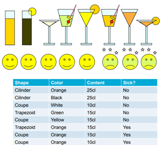
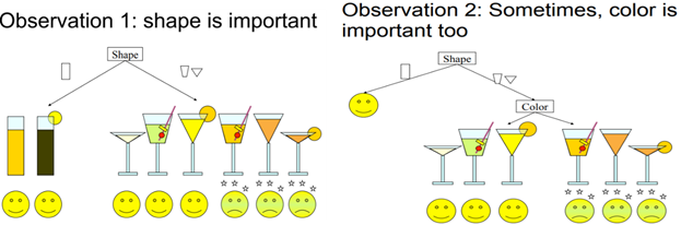
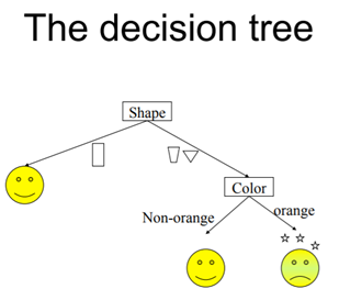
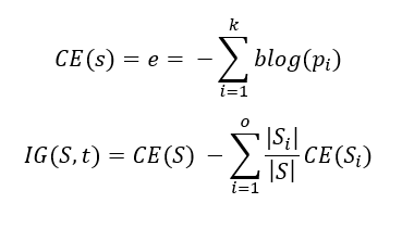
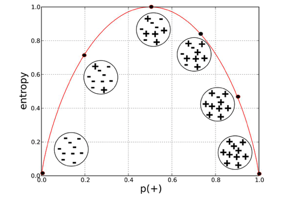
All the drinks that come in cylindrical glass or if they are in any other shaped glass then it should be non-orange for it to be safe. The above diagram shows us how we can separate bad drinks from good ones, but we did this visually, how to do it mathematically then? We need to decide which feature should be put in which node, to do this task, we use something called information gain or Gini index (Impurity measure). The first thing that comes to mind when you hear entropy is chaos and it is exactly that. We need to build the tree in such a way that it reduces the entropy of the system or increases the information gain at every child node creation. Given below is the equation of entropy, (blog is log with base 2 or binary log). To be precise entropy is called class entropy (for DT) and using this we calculate the information gain. Information gain is the expected reduction of entropy if we add a certain feature as the condition in a given node at a particular depth. Let’s understand this with an example. But before we go further let’s understand another term called Gini Index.

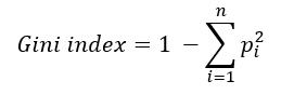
The Gini index is a measure of inequality in the sample. For practical purposes, we use the Gini index rather than information gain. It has a value between 0 and 0.5. Gini index of value 0 means samples are perfectly homogeneous and all elements are similar, whereas, Gini index of value 0.5 means maximal inequality among elements. It is the sum of the square of the probabilities of each class.

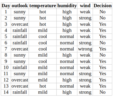
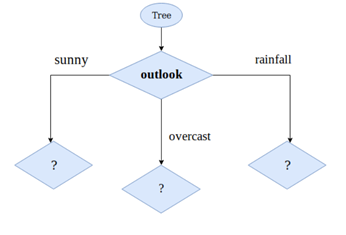
Let’s try to understand the Decision tree through our toy dataset 2 which is shown in the above table. This dataset tells us when can we go for a wonderful tennis match and when we can’t. We have 5 features here namely outlook (Sunny, overcast, rainfall), temperature (hot, mild, cold), humidity (high, normal), and wind (weak, strong), we need to select one feature from these 4 features that will be our first root node. This feature will produce the maximum reduction in the entropy. First, we are going to see the feature outlook and calculate the Gini index for its categorical value (sunny, overcast, rainfall, and overcast).

Out of 5 sunny in the above table, we have 3 Yes and 2 No. So, our Gini index is calculated as given below:

Gini index (outlook=sunny)= 1-(2/5)²-(3/5)² = 1- 0.16–0.36 = 0.48

Simlarly, we calculate the Gini index for other 3 categories of feture Outlook.

Gini index(outlook=overcast)= 1- (4/4)²-(0/4)² = 1- 1- 0 = 0

Gini index(outlook=rainfall)= 1- (3/5)² -(2/5)² = 1- 0.36- 0.16 = 0.48

Once the Gini index of each category in a given feature is calculated, we calculate the weighted sum of the Gini index for the feature outlook. Here have 5/14 proportion of sunny, 4/14 proportion of overcast and 5/14 of rainfall, give below is the calculated value of weighted Gini:

Gini(outlook) = (5/14)*0.48 + (4/14) *0 + (5/14)*0.48 = 0.342

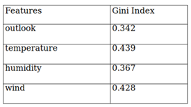
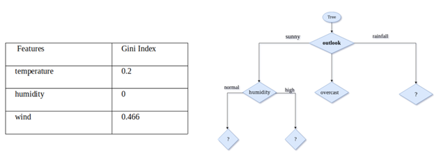
We follow the exact same procedure for temperature, humidity, and wind. Results for all 4 features are shown in the table below. From the below table, we can see that the Gini index for the outlook feature is the lowest. So, we get outlook as our root node.

We repeat the same procedure, but this time we look at sunny, overcast, and rainfall sub-data. First, we calculate the above table results when the temperature is sunny, then for overcast, and then for rainfall. Doing this for sunny we get that humidity gives us the lowest Gini index so we choose humidity to split our node. we keep doing this process until the validation accuracy is increasing or all our features are exhausted.

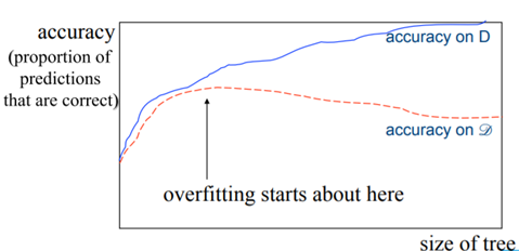
After a certain depth Decision tree's accuracy starts decreasing. We need to be cautious of not overgrowing our trees as they can easily overfit after a certain depth which is showcased by the above graph. Here’s another question, when should we stop growing the tree?

We have two options with us, cautious splitting and post-pruning. Cautious splitting is that we try to guess the accuracy of the unseen data, it is basically validation data accuracy. Post-pruning is training a full tree and then remove the nodes which have very few elements in their leaf nodes or if cutting that node doesn’t lead to a huge change in the accuracy. Not pruning is usually a very bad idea (most of the modern DT algorithm implementations already have pruning in built-in them)

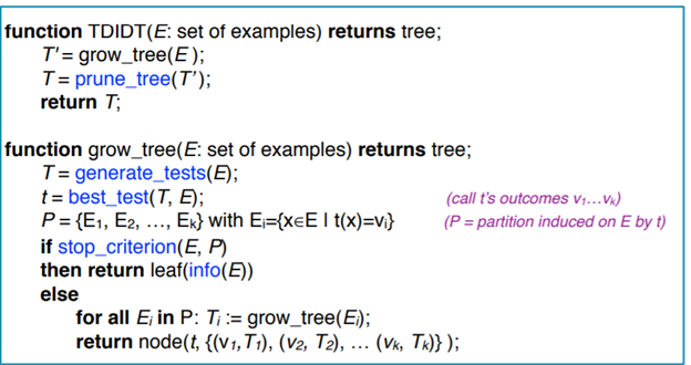
Here’s the full pseudo code for top-down-induction-decision-tree. Generate test and then chose the best test (from all the impurity measures choose the one which gives you the best result). Partition the data based upon the best test and keep growing the tree until the node became a pure node (all elements in a node belong to the same class). And finally, prune the tree to avoid overfitting.

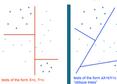
What we showed above was meant only for categorical data, but this technique works even with numerical data. For numerical data, we just need to introduce the threshold term for every feature. We calculate the Gini index of a feature by sorting the feature and then applying a threshold to every value in that feature and then choosing the feature with the lowest Gini index as the candidate for the root node. Generally, the decision tree produces an axis-parallel decision boundary, but we can fit oblique lines also by changing the best_test in the above pesudocode. Given below images shows the result for both axis parallel and oblique trees.

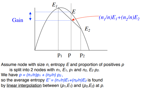
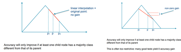
One last thing about decision trees is that they should always have a strictly concave impurity measure. The below diagram shows how’s gain calculated. If the impurity measure is not concave (see the triangular case), then even for different proportions of positive and negative sample gain will still remain zero. We will only get gain when one of the child nodes has a different class than its parent’s node in the case of the non-convex impurity function. (Read the text written in the below image properly to understand the concept of strictly convex impurity function)

I hope now you know a little more about the decision tree, if anyone of you wants the code for the decision tree from scratch comment down below. And also suggest what do you want to learn next.

HAPPY LEARNING…