Deep Reinforcement Learning: Toward Integrated and Unified AI

Can AI provide a lens on human intelligence?

Most artificial intelligence(AI) models today, including convolution neural networks (CNN) and large language models (LLM), are built for specific tasks and require humans’ curation of vast training data. They lack the capability to interact with the world or to learn continuously. However, deep reinforcement learning (RL) stands out as one shining exception, showing scalable self-learning without supervision. An RL model has an agent that learns from its interactions with the environment to maximize rewards, the behavior mimicking what animals do in natural environments. This intersection between engineering and psychology also makes RL an ideal model for discovering the brain’s underpinnings of reward-based learning and decision-making.

RL was born in the 1950s and has undergone significant enhancements ever since. Notably, American mathematician Richard Bellman first established the theoretical foundation with Bellman equations and the dynamic programming algorithm (DP). In the 1980s, Canadian computer scientist Richard Sutton and his PhD adviser Andrew Barto introduced temporal difference learning (TD), which scaled up the learning process tremendously. In the 2010s, British computer scientist David Silver and his team in DeepMind integrated deep learning into RL, reaching a pinnacle in AI history — DeepMind’s AlphaGo beat the world champions consistently with astounding super-human performance.

As of today, RL’s progress hasn’t slowed down. Its flexibility in unifying various models and methods driven by the simple behavioral protocol has made it an excellent candidate for further AI integrations. In parallel, it also provides theoretical testbeds for studying how our mind drives complex cognitive behaviors.

The purpose of this article is to better understand where RL’s unifying power came from and what impact it has had on our comprehension of the biological brain. We will first take a broad stroke on the theoretical foundations of RL, before diving into deep reinforcement learning to appreciate the power of AI integrations. Subsequently, we will examine how the RL theory explains dopamine neuronal signals in animal reinforcement learning. Lastly, we will explore how RL may be used to simulate and shed light on multiple decision-making systems in the brain.

What is Reinforcement Learning?

Reinforcement learning was started from the engineering quest for decision-making. Psychology and neuroscience do not use the term to describe animal or human behaviors. Instead, they use more specific terms, such as classical condition and instrument learning, all of which involve reward-based learning, and the reward is sometimes called the reinforcer.

Given the interdisciplinary nature of this article, we will only touch upon the general features of RL that draw inspiration from psychology and neuroscience, with minimal mathematical equations. For more details on RL, I highly recommend the book Introduction to Reinforcement Learning by Sutton and Barto. Readers can also find excellent articles on mathematical deep dives on Medium.

Iterative Sequential Learning with Delayed Rewards

The RL problem is simple and intuitive. It consists of a software agent and an environment in which the agent makes observations and takes actions to obtain maximum rewards. Realistically, the reward is usually delayed and given at the end of a sequence of actions. For example, in a typical video game or chess, you have to execute many steps and overcome many obstacles before knowing whether you have won or lost. It’s the learning by trial and error that an RL needs to solve.

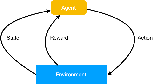
In contrast to supervised learning (SL), where each sample is labeled with the desired result, an RL agent learns whether its actions are good or bad from reward signals. Furthermore, time matters in RL because the agent makes a series of decisions, each affecting the subsequent data it receives. After many trials and mistakes, the agent will eventually determine the optimal series of actions to obtain maximum rewards.

From the beginning, RL is based on two fundamental mathematical assumptions: first, an RL problem consists of a sequence of states, one leading to the next; second, the sequence can be treated as iterated steps of solving the current state and its immediate next state. The former is called the Markov Decision Process (MDP), and the latter is represented by Bellman equations.

A state includes the information given by the environment for the agent to determine what happens next. The Markov premise is that every state (at a given time t) determines the next step (at time t+1), which is expressed as:

This means that, given the present, the future is independent of the past. Once the state at a given time is known, the history before it can be ignored.

Likewise, a state is a sufficient statistic of the future. Because the environment gives the rewards, the following state (t+1) includes the accumulated reward from the future.

Now, let’s look at the agent. An RL agent has two functions: policy and value function. Policy is the function of the agent’s behaviors, essentially a map from state to action as:

A value function predicts the future rewards to evaluate the goodness or badness of each state. While a reward signals what is immediate, a value function specifies what is good in the long run as the total reward an agent can expect over all the future steps given the current state.

Here, gamma γ is the discount factor between 0 and 1, considering the immediate reward has a higher value than the future reward. There are multiple reasons why the discount factor makes sense. Psychologically, humans generally prefer immediate reward over delayed reward. Mathematically, it is convenient to have the equation converge to a maximum reward. Furthermore, because we rarely have a perfect model of the environment, the discount factor takes the uncertainty into account.

Given the MDP property, the above value function can be re-written as:

The agent’s problem, therefore, becomes a step-wise recursive process that seeks the action with the maximum future value, as predicted by the value function for the immediate next step. This operation is called the Bellman equation, generalized as:

Similarly, the action-value function becomes:

Next, the well-known Q function determines the action that will return the maximum future rewards.

Essentially, Bellman equations provide the mathematical method for the agent to learn the optimal sequence of actions with iterative steps through decomposing the valuation function and policy into subproblems of the current state and the immediate next state. Bellman called this process dynamic programming (DP).

DP works nicely to solve engineering problems where the environment is fully understood, and there are limited action steps. However, it would fail to solve the problem of a novel environment with numerous possible states.

Temporal Difference Learning by Predictions of Rewards

An alternative to DP when facing an unknown environment is Monte Carlo (MC) sampling, which allows the agent to take random sequences of actions and update its value function and policy with incremental learning.

In contrast to DP, the MC method does not require prior knowledge of the environment’s dynamics. This is like exploring a new environment when we hike without prior knowledge. We can try a few directions and follow each one from the start point to the destination. After following each path, we will record the time it takes and score the road condition. Obviously, another advantage of the MC method is its ease and efficiency of going through a small subset of states instead of accurately evaluating the entire state set in DP.

However, for many realistic problems requiring a long sequence of possible steps before receiving the rewards, the MC method means the agent must traverse every step from the beginning to the end before learning and improving, which could be costly and extremely slow. Instead, Sutton’s temporal difference (TD) method makes the learning happen much earlier from the prediction errors at each step, in which the value function is updated based on any violation of predictions instead of actual actions.

Suppose I need to drive from Long Island to New Jersey in the shortest time to make an appointment. On the way, I notice my estimated arrival time is longer than the target. I base my estimate on the current position and decide to take a different route to minimize the estimated delay. After I get on the alternative route, my estimated arrival time is now on target. My decision based on my estimate is correct. If not, I may continue to adjust until I find the quickest route to reach my destination. This is an example of TD learning from predictions instead of actual mistakes at destiny when it would be too late.

TD makes learning entirely online by incrementally updating estimates based in part on other learned estimates without waiting for a final outcome. In other words, the efficiency comes from learning a guess from a guess.

Like DP, TD is simple to implement by leveraging the MDP process. It only needs to update the value function and policy incrementally at each step based on the estimates of the total future value. Therefore, it has become the most widely adopted RL method today. Interestingly, as our intuition tells us, our brains may also use TD learning in many situations (as in the example above). With inspiration from Sutton and Barto, neuroscientists have found the biological mechanisms exactly as the TD algorithm has illustrated. We will come back to this in detail in a future section.

Model-based Planning

RL can optionally incorporate a model to predict how the environment delivers the reward and transitions from one state to the next, if the environment is fully known or reasonably understood. The original Bellman’s DP method requires a perfect model of the environment, whereas the MC and TC methods don’t. DP is a model-based method, while MC and TC are model-free.

For an unknown novel environment, a model-free RL with TD is effective for the agent to learn by trial and error. It mimics animal reinforcement learning behaviors initially discovered in cats and fish by American psychologist Edward Thorndike(for more details, please refer to my previous article on the evolution of decision-making). As an RL problem becomes complicated with many steps, the model-free TD needs to be more efficient since it still relies on interactions with the environment. In this case, using a model with the learned rules to simulate the agent’s experience and enable it to plan ahead could further reduce the learning time.

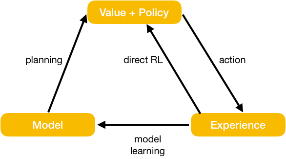
We can use the same example of driving from Long Island to New Jersey mentioned previously. Suppose I have already studied the map and know most routes from Long Island to New Jersey, including the time each route takes. When I expect a delay on my current path, I could do a mental search among multiple alternative routes to find the best one. This would be much more efficient than simply trying an alternative route. It means I have a model that allows me to do model-based planning.

The advantage of having a model is that it allows an RL agent to do simulations using the model outputs instead of direct interactions with the environment. The savings can be significant. As shown in the above chart, the simulations depend on the agent’s understanding of the environment. Therefore, a model-based RL usually includes model-free TD learning with real experience. A balanced mix of both types of learning is critical to the success of RL.

A great example of model-based RL is AlphaGo, in which DeepMind implemented a forward search algorithm named Monte Carlo tree search (MCTS). The model generates simulated moves for AlphaGo to play against itself (instead of playing against the opponent player). The simulations were essential for AlphaGo to eventually beat human professional players in the full-sized game of Go in history.

Deep Reinforcement Learning

In a natural environment, animals move around and observe the information based on their locations and where their eyes are directed. The raw sensory information that the eyes have gathered is then processed through the visual neural networks in the brain. The output includes the higher-order classifications and feature concepts formed in the visual cortex, enabling the animals to judge the situation and make decisions quickly.

The early RL models lacked this capability of sensory information processing, preventing agents from learning in realistic environments. In the 2010s, DeepMind published its first deep reinforcement learning model, in which a deep CNN was added to the RL model to learn directly from visualizing the computer screen and guide the agent’s actions for the rewards. They used this model to play the Atari 2600 video games. The results were ground-breaking. With the addition of deep CNN, the same model could learn all seven Atari games tested. It outperformed all previous RL algorithms in six games and surpassed an expert human player in three.

CNN is a typical type of supervised learning. It requires large training sets of hand-labeled images. In the case of Atari games, the RL takes sensory information and reward signals from the computer screen and trains the CNN to learn the value function. In other words, the deep RL eliminates the preparation of manual training sets and replaces it with a behaving agent to acquire the data from the environment by taking incremental actions. Deep RL was a significant leap in AI self-learning, particularly considering that RL learning depends on reward information that is usually delayed and noisy.

Another main difference between a conventional CNN and deep RL is that data samples for supervised learning are independent of each other, whereas they are usually highly correlated in RL because sequential movements lead to highly correlated states. Furthermore, because the expectation of rewards drives the agent’s behavior, the sequence of actions can sometimes lead to drastic changes in sample distributions when a new behavior pattern is introduced.

Given these challenges, the DeepMind researchers made another addition — the experience replay — to feed the CNN with random samples from past episodes stored in the memory. The replay effectively smoothed the sample distributions and made the CNN converge on learning the most salient features that would yield the maximum rewards. Notably, the replay was offline when the agent was not interacting with the environment to avoid conflicting information feedback from the actual actions.

The above CNN and experience replay have presented a refreshing similarity to how the brain works with integrated computations across multiple regions. We learn by seeing while navigating in an environment. Our memories are then consolidated and stored for the long term after offline relays during deep sleep, as reviewed in my previous article on memory and forgetting. The success of deep RL is another instance of innovation inspired by the biological brain.

Dopamine and Temporal Difference Learning

In the 1980s, neuroscientists became intensely interested in RL, particularly the TD method implemented by Sutton. Their collaboration with Sutton led to the discovery of dopamine’s computational role in reward-driven learning in the brain, a perfect example of the convergence in AI and neuroscientific research.

Deep in the midbrain of all vertebrates is a dorsal striatum consisting of dense clusters of dopamine neurons. These neurons send their output to many brain regions, including the neocortex, and have long been linked to rewards. However, its exact role in reward-based learning was not clear.

The initial hypothesis was that dopamine delivers the pleasure signal that makes animals feel good. In the 1950s, German neuroscientist Wolfram Schultz was the first to measure the activity of individual dopamine neurons during simple learning tasks. His experiments proved that dopamine neurons do not respond to the reward itself (e.g., sugar or food). Instead, they respond only to the predictive cues leading to the reward, not the cues without following rewards. Schultz’s data suggested that dopamine may be related to wanting or predicting the reward.

In 1997, inspired by Sutton’s TD theory, neuroscientists Dayan and Montague aimed to re-interpretate Schultz’s findings. Their experimental data and theoretical calculations proved that the dopamine neuronal activities signal the animal’s predictive errors, which can be precisely described by the TD algorithm. In other words, the brain is able to calculate a reward prediction error, which in turn triggers the release of dopamine to induce learning.

In 2013, another paper published in Nature by DeepMind and neuroscientists from Harvard made another significant step. They demonstrated that for more complex behaviors with multiple reward options, the population of dopamine neurons encodes the probability distributions of expectation errors for different outcomes. The encoding could also be quantitatively described and explained by the distributed TD theory.

In summary, the quantitative proof of dopamine’s role in temporal difference learning is one of the few theories supported by empirical data in neuroscience. The discoveries represented some of the most fruitful partnerships between AI and neuroscience. They signify a leap in history toward a deeper understanding of how our mind works — when our behaviors are guided by internal prediction or anticipation of a rewarding outcome.

Thinking Fast and Slow: Model-free vs Model-based Learning

As previously mentioned in this article, RL has two distinct types: model-free and model-based. The latter allows the agent to leverage a world model to plan before deciding its next best moves. Over the last decade, model-based RL has become an exciting field for studying how humans make goal-oriented decisions.

We know humans can plan using imagination. In other words, humans behave as model-based RLs capable of playing out different options in their heads before making the predicted best moves. However, exactly what kind of models humans use in their minds is a hot topic actively pursued in psychology, neuroscience, and cognitive science.

The Nobel laureate and prominent psychologist Daniel Kahneman described the conflicting System 1 and System 2 in his famous book “Thinking, Fast and Slow.” System 1 is fast, automatic, and intuitive, while system 2 is deliberate and slow. Kahneman admitted that no magical resolution exists to enhance System 2 except through education and systemic training. In light of deep RL, System 1 is likely the result of model-free RL learning, which is biased and inflexible to change once learned. Conversely, System 2 has a model of the world, which enables humans to be more thoughtful with mental planning and simulations.

The “dual” systems also manifest at the behavior level as automated habits vs goal-directed controls. Studies have demonstrated that a habit results from a model-free RL after extensive training. The learned behavior persists even when the reward is diminished or removed. Conversely, for a model-based RL, the brain can adjust the behaviors quickly when the reward is changed. In other words, model-based RL is more flexible when coping with uncertainties in an environment.

Moreover, an RL can be model-free and model-based simultaneously. As stated by Sutton and Barto in their book, a state-of-the-art RL agent performs the best when its learning combines model-free trials and errors and model-based planning. This gives us a different lens to view the relationship between the two systems more deeply — an area where their simultaneous competitiveness and cooperativeness could be unified. RL could become a unified model to explore the dynamics of both processes and unlock the computational underpinnings of human “fast” and “slow” decision-making.

Conclusions

We are in an era when AI is making remarkable progress that is both exciting and unsettling for humankind. Among the successful AI models, RL is unique in its simple behavioral paradigm, mimicking animal and human learning with trial and error to seek the most accumulated rewards. It has achieved remarkable super-human performance in the past few decades, particularly in games, after integrating and unifying with deep learning and brain-inspired methods.

The strength of RL lies in its ability to self-learn any arbitrary behaviors (as opposed to human-curated training data) and its flexibility in integrating and unifying different modules and processes. Besides integrating with deep learning, another example is the coexistence of model-free and model-based learning, an excellent candidate for generalized fast learning.

The history of RL has also shown the beautiful partnership between AI and neuroscience. RL has provided proven quantitive theories to explain dopamine’s role in signaling prediction errors in the brain. The collaboration will likely accelerate in the coming decades, and we expect to see more ground-breaking insights into the inner workings of human minds.