DEEP DETERMINISTIC POLICY GRADIENT FOR CONTINUOUS ACTION SPACE

In the previous article about Policy gradient methods, we discussed the shortcomings of PG-based methods. They are not sample-efficient as they discard the previously learnt policy in each iteration. We can say they are on-policy learning methods as the same policy generates the action and updates the value function. These methods don’t utilize the value function information, which requires an off-policy setting. So we have a new set of algorithms called Actor-Critic methods and DDPG is one of them.

• Policy gradient is preferred over value-based methods in the continuous space domain, as they don’t solely depend on the value function of the next state (like in 1-step TD learning) for optimization. They have a scoring function, which improves by taking actions that maximize our rewards. But we need to mix the best of both worlds (Value-based and Policy-based methods) to build algorithms.

LIMITATIONS OF VALUE-BASED METHODS

• Algorithms like DQN, utilize the value functions of state V(s) or Action value function Q(s, a). These algorithms work in the discrete space domain. But the curse of dimensionality always kicks in discretization. In the paper, the authors give an example of the human arm

For example, a 7 degree of freedom system (as in the human arm) with the coarsest discretization aᵢ ∈ {−k, 0, k} for each joint leads to an action space with dimensionality: 3^₇ = 2187.

• Such large action space is difficult to explore efficiently and methods like epsilon-greedy come with more hyperparameters to optimize and keep track of. Additionally, naive discretization can lead to sub-optimal results. So DQN scales to high dimensional observation space like images from Atari games, but not to high dimensional action space, PG methods are a better alternative. So let's get into DDPG which combines the best of both worlds.

BUILD-UP TO DDPG ALGORITHM

• DDPG (Deep deterministic policy gradient) is a model-free off-policy Actor critic method.
• In actor-critic algorithms, we have 2 sets of function approximators (which can be neural networks). One set is called the actor which is based on policy gradient methods and the other is called the critic which determines the value function of a state. So like in real life as a critic analyzes the actions of an actor and gives reviews, now the actor has to take actions to impress the critic. As the critic gets a better view of the world, so as the actor based on the review of the critic

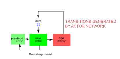
• Also, another data structure we use in the Actor-Critic network called Replay Buffer. It is a deque and it stores the transitions generated by the actor-network plus some noise for exploration as a tuple (s, a, s’, r) where s is the current state, a is the action taken at state s, s’ is the next state and r is the reward after taking action a in state s.
• We require a replay buffer to satisfy the i.i.d (Independent and identically distributed random variable) condition for neural networks. Like each time you toss an unbiased coin, both head and tail have equal chances of happening and the next toss result is independent of previous tosses. So i.i.d assumption states the conditional probability of p(yᵢ|Xᵢ), where model prediction of yᵢ is dependent on Xᵢ only, not the relation between Xᵢ and Xⱼ (Xᵢ and Xⱼ being different data points).

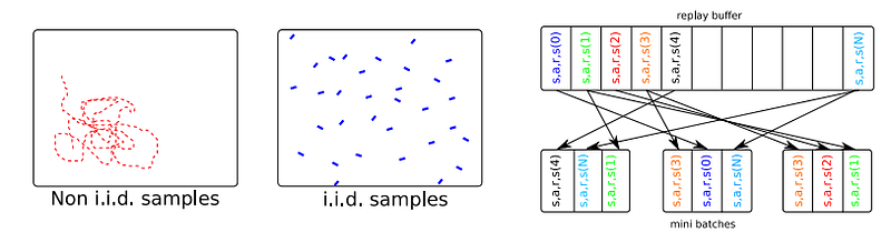
• Non-i.i.d samples are sequential data generated from actions taken from the actor-network. If our model learns from this set of sequential samples, then it voids the i.i.d assumption. So to preserve the i.i.d assumption we generate transitions and save them in the replay buffer and while calculating the error we generate a random mini-batch. DDPG is an off-policy algorithm, the replay buffer can be large, allowing the algorithm to benefit from learning across a set of uncorrelated transitions.
• First, let’s define the action-value function, it represents the expected return from taking an action aₜ in sₜ and thereafter following the policy π

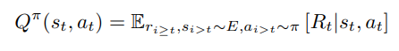
• Here, E is the environment and π is the policy. [Rₜ|sₜ,aₜ] gives the reward you get from the environment after executing the action aₜ in state sₜ.
• [Rₜ|sₜ,aₜ] gives the discounted reward till we reach the end of episode or number of pre-defined time steps (in a never-ending episode). The above equation can be written in a recursive form

• So it is the summation of the reward you get after executing the action aₜ and estimated Q-function of the next state Sₜ₊₁. So as your estimates for states get better, your estimate for the next step also get better (vice-versa)
• The second term is known as the target term, it has a close resemblance to the TD learning target and in implementation, we have a separate target network that spits out the Q-function of the next state. Deterministic name in the algorithm DDPG comes into play now, the target is deterministic as it is defined by our actor policy plus some noise (Ornstein-Uhlenbeck noise). So we can get rid of the expectation

• The Ornstein-Uhlenbeck noise implementation in Open AI baselines. Ornstein-Uhlenbeck is part of the stochastic differential equation. To ensure that we have sufficient exploration among the action space and our actions being part of the stochastic process.

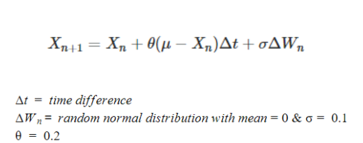
• Here Xₙ is the distribution of all possible action space and it is of the same shape as μ. μ is of the shape (num_actions,1). Wₙ size is identical to μ and can be implemented by numpy.random.normal.

TRAINING ACTOR AND CRITIC NETWORK

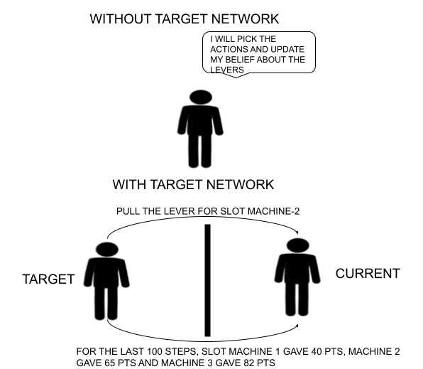
• In DQN, we have a target network and a current network. So we generate transitions and store them in a replay buffer → Initialize the weights of both target and current network → target network are held fixed and the current network learns from the estimate → at regular intervals (a hyperparameter) clone the weights of the current network to target network. So why do we need a target network?
• If the same network is selecting the action and updating the value function, it will lead to overestimation. For example, in a slot machine, if you pull a lever and get a high reward then you will keep on pulling the lever and overestimate the reward that you will get from the lever as you are fully aware about the environment. So here selecting an action and updating the belief about the lever are coupled.
• Now suppose you bring your friend and assign him the task of selecting the action for you and you will update him on the reward that you get at certain intervals, you will update your belief about the levers based on the actions instructed by your friend. So decoupling these two tasks can lead to sufficient exploration (you can instruct your friend to be random at selecting action). Also, in Q-learning we take the max of the action value function in the next step, when your estimates are bad then you may build on top of your bad estimates and by taking max you can overestimate. So if you choose another network (Target) to select actions for you, then you can ameliorate overestimation.

NOW COMING TO DDPG

• To train the critic network in each time step for N samples in a mini-batch

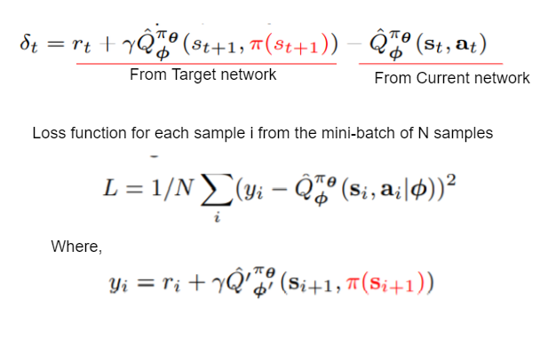
• Note here, π(Sₜ) means the action taken by the target actor policy. aₜ is defined as current actor policy plus some exploration noise. It is part of the behaviour policy which generates transition to be store in the replay buffer.
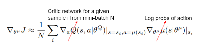
• To train the actor-network, we follow the policy gradient theorem

• We have a target and a current network for both actor and critic. In the ablation study, the authors show that both are essential for getting superior results. Rather than playing with a hyperparameter (RL algorithms are sensitive to seed values and hyperparameters), we have a soft update rule

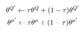
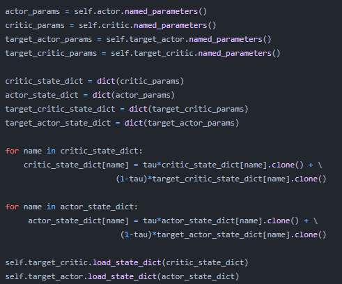
• As tau<<1, the target networks have a stable and slow update ameliorating the divergence problem. Also, a soft update ensures that we have a relatively fixed target. The python implementation would look like the following (Note: If you use LayerNorm here instead of batch normalization, then the below code is valid).

• Also, the authors mention batch normalization because different components of observation have different units and range like velocity, position, angle etc which would affect generalization. So to scale these features, batch normalization is used for all layers prior to the output layer for both actor and critic network. It maintains a running average of the mean and variance of a minibatch and minimizes covariate-shift (different distribution of train and test set).
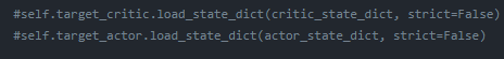
• You can use layer norm instead of the batch norm. Layer norm normalizes for a layer, not a mini-batch. The only change you need to do in the above code if you are using batch normalization is

CONCLUSION

• DDPG solved some problems in Policy gradient and Value-based methods.
• Policy gradient methods are sample-inefficient, they always start fresh and discard the previously learnt policy. They don’t utilize the value function information of a state. DDPG which is an off-policy algorithm is sample-efficient as it has a replay buffer that stores the previous transition, whereas in Policy gradient we are at the mercy of the stochastic policy to generate the previous transition again. Target network keeps track of the previously learnt policy by the soft update rule.
• In the value-based method, we were unable to scale to a continuous domain without proper discretization. Also, with sufficing discretization curse of dimensionality kicks in and we are at the mercy of epsilon greedy strategies to explore the entire action space. Epsilon-greedy comes with more hyperparameters to optimize.
• However, DDPG has some limitations. It requires a lot of training episodes to converge and generalize. Non-linear function approximators like neural networks help RL agent to generalize to multiple tasks, so we are set on the right path but we need more robust algorithms to converge faster.