POLICY GRADIENTS IN DEEP REINFORCEMENT LEARNING

In 2016, a deep learning Reinforcement agent AlphaGobeat Lee Sedol, who is a professional Go player of 9 dan rank (the highest honor in the field of Go). Go was regarded as a game far-fetched from computer algorithms because it has an artistic essence to it. But AlphaGo, developed by Google DeepMind was able to beat Lee Sedol 4–1 in a 5-match series. This event really sent a shrill to human intelligence all over the world, it becomes apparent from the fact that Lee Sedol took a cigarette break during one of the matches.

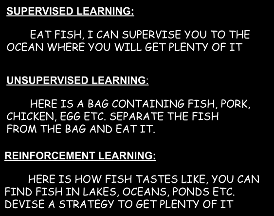
Reinforcement learning, unlike Supervised learning, works based on a reward function compared to data labels. In Reinforcement Learning, we have state, actions and rewards. The agent has to come up with a strategy to maximize its rewards. An RL agent has two components, i) description of the state based on Value functions, ii) policy distribution. The first one has algorithms like Q-learning, DQN, DDQN etc. The second one has different algorithms which we are going to discuss in this article.

LIMITATIONS OF VALUE-BASED METHODS

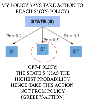
• The policy is simply mapping a state to different possible actions. So given our state, which action to take so that going forward we can maximize our reward.
• In the value-function method, first, we randomly choose a policy and you are dropped at a random state, then following that policy we estimate how good are the states that we are visiting. The states that give higher rewards going forward have a higher value function. So while building your final policy, you will choose states greedily (also you need to explore sometimes by choosing a state randomly by introducing some noise to our pre-defined randomized policy while learning).
• But sometimes it is better to learn a policy than accessing the quality of the state. Drawing parallels to real-world, given your present conditions, you are better off if you know what to do rather than how good or bad your present condition is.
• Also, value-based methods are not feasible in continuous action space. Here given a state, we need to pick an action that maximizes our action-value function. Algorithms like Q-learning are great with higher observational state spaces like Atari games which have 80x80 (image dimensions) state space, but they cannot handle higher dimensional action spaces. In the paper DDPG, the authors give an example of the Human arm which has 7 degrees of freedom and even if we will consider 4 possible actions (up, down, left and right) in each DOF, we will 4⁷ = 16384 possible action space. It is difficult to explore all these actions with techniques like epsilon greedy.
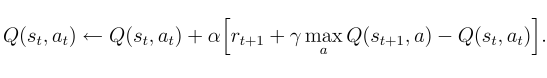
• Q-learning methods work by minimizing the TD error between our estimate of reward along with the action-value function of NEXT STATE (Sₜ₊₁), and the action-value function of the present state. But in the continuous domain, NEXT STATE (Sₜ)needs proper discretization so that we are not throwing away a lot of information and it is hard to achieve.

• So to ameliorate these problems, we should try to learn the policy of an agent rather than only considering the value function. PG methods have their own set of problems, so a new set of Algorithms called Actor-Critic are developed which consider both policy and value functions. But here we will concentrate on PG methods, particularly REINFORCE.

POLICY GRADIENT METHODS

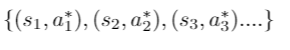
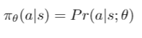
• First, a policy is defined by the probability distribution corresponding to each state. Consider a supervised setting, here policy would be (state, optimal action) pairs, where we map a state to an action that would maximize our reward. But we need an oracle or a human annotator for this mapping. So in the Reinforcement learning setting, we have a reward function that can train the agent to pick actions that maximize reward.

• Remember, in limitations of value-based methods, we discussed exploration of state space and strategies like epsilon-greedy comes with more hyperparameters to tune and optimize. Policy gradient tackles this by having a stochastic policy, where exploration is built into our policy. Probabilities ensure that all actions are probable to be included in our policy, not like a deterministic policy where we have one-hot encoded type probability distribution.

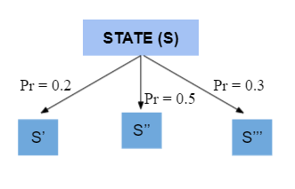
• So a policy tries to determine the probabilities of going to all possible future states. If an action leads to a state that maximizes reward going forward, the probability distribution at the current state should assign a higher probability to that action. But to determine the optimal action, the probabilities need to be tied to a scoring function (higher the score → higher the probability).

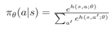
• The scoring function, which is approximated by any function approximation, tries to assign higher probability values to optimal actions. Neural networks are generalizable function approximations.

Now how to design the scoring function and what it should try to maximize?

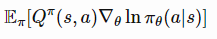
• We should design these functions so that they maximize the rewards. The stochasticity at each state will enable us to explore all possible action space and choose the optimal one. To maximize our rewards, we can use ACTION VALUE FUNCTION Q(s, a; θ). Q(s, a; θ) is defined as the discounted sum of rewards when starting in state s, executing an action a and then following our parameterized policy by θ.

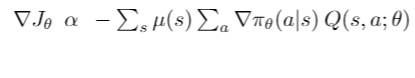
• Here J is a proxy for our scoring function, so we want it to be MAXIMIZED → GRADIENT ASCENT (hence you see negative in the gradient update)
• μ(s) is the stationary distribution state or how many times you visited state s while following your policy. It turns into expectation value. The expectation value is calculated when you cannot consider the population mean. Like calculating the average height of the population is infeasible, hence we randomly sample a batch of population and take the average. According to the law of large numbers, the more you visit a state, the better your estimates are. But we cannot visit a state more often, hence we take an expectation value (which serves as a satisficing estimate).
• Now, we know that summation of probabilities of all possible actions is 1, hence we can divide and multiply the policy distribution (it sums to one because there is a summation operator)

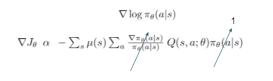
• The θ in the action-value function is omitted, rather we have a superscript π, which tells that the Q function estimated based on our current policy parameterized by θ (On-policy).

REINFORCE MONTE-CARLO ALGORITHM

• In Monte-Carlo, the discounted rewards are accumulated till the end of the episode, it is denoted by Gₜ

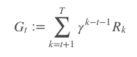
• Gₜ replaces Qπ(s, a) in our gradient ascent equation and we update our policy in each time step. This algorithm is known as REINFORCE MONTE-CARLO. The pseudo-code for these algorithms is taken from this video

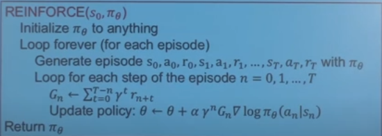
• So you initialize a policy π_θ, by randomly initializing probabilities for each action in each state → for each episode, generate transitions following your randomly initialized policy and save those transitions in your replay buffer→ for each time step of the episode (initial state to terminal state), calculate the discounted reward Gₙ → you can grab a batch of transition (to calculate the batch loss) and then update your policy (see the gradient update is positive because we included minus in gradient ascent step).
• Also, note here, θ is higher if your Gₙ is higher and θ is proportional to the probability of action in a given state. As our agent plays more episodes, it builds a good estimate of our environment states that is Gₙ, so as your policy. In short, the action for which Gₙ↑ → θ↑ →Pr(optimal action)↑.

BASELINES TO REDUCE ESTIMATION ERROR

• Monte-Carlo estimates generally have high variance. Bias and Variance have an inherent trade-off. If your model overfits your training data, then it would have a low bias (low training error) but high variance (high test error). So in Monte-Carlo, we sample a whole episode and then take average to update our value function. So your agent will get good at the current trajectory which will decrease bias, but your variance would increase, because it may fail in another trajectory. Also, your estimates may not be accurate during the initial stages of training. So you would have noisy estimates and erroneous gradient updates which would accumulate.
• To mitigate these problems, we have the concept of baselines. Baselines try to reduce the error in our estimates and address our Q-function. First, let’s understand the Value function (V(S)).

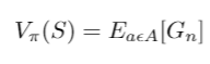
• Value function gives the expectation of all the discounted rewards that you will get after taking an action according to your policy. It is an expectation because these are estimates, not true values, as you train more your estimates gets accurate. So it gives an average interpretation of how good the state is so that we pick states with higher value function. Action Value function Q(s, a) is defined by

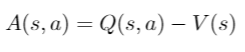
• Action Value function gives how good an action is given a state. So Q(s, a) caters to one action and V(s) caters to the average of all actions in a given state. Now, we define the Advantage function A(s, a)

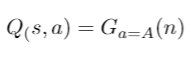
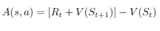
• We can also write Q(s, a) as Gₙ because the latter gives the discounted reward of taking an action (it is just the Monte-Carlo estimate). If you want a temporal difference update, you can do

• Advantage gives the relative advantage or disadvantage of an action over the mean. If your Q(s, a) is more than V(s), then those actions are better than average (we should encourage our agent to assign higher probabilities to these actions) and vice-versa.
• Also, V(s) does not depend on the action a, hence it won't affect our gradients as the gradients are taken w.r.t to a.
• So now getting back to our Monte-Carlo REINFORCE algorithm with BASELINES

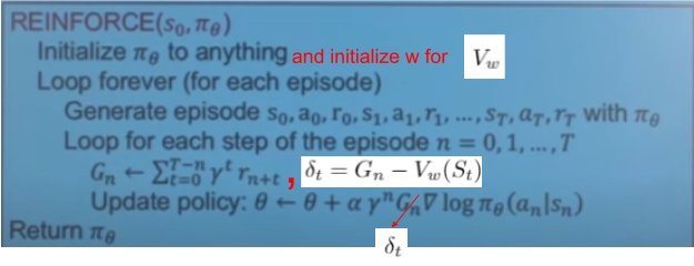
• Your θ is proportional to δt if your action is better than average then you have a higher probability of getting selected.

LIMITATIONS OF POLICY GRADIENT

• Policy gradient methods are not sample efficient. Policy iteration methods are on-policy methods, hence they discard the previously learnt policies. Value function are sample efficient because they retain information about the states, which could be used by the agent to derive a policy. So Actor-Critic algorithms, which have both policy and value evaluation, are more sample efficient. In on-policy, the agent uses the same policy to estimate and evaluate the value function and in off-policy, the agent uses different policy for evaluation and estimation.

• Policy gradient methods are not generalizing, as we train our agent in our given environment, the stochastic agent eventually becomes deterministic. If we translate the agent to another surrounding, it won’t perform well Drawing parallel to real-life of learned helplessness, if you are spoon feed about what to do given a situation, you may end being too much dependent and not perform well in other challenging life tasks.
• It is susceptible to local optima. PG methods don’t use state value functions, hence they may converge to local optimum points.

This wraps up PG iteration methods in Reinforcement, we first looked into shortcomings of value-based methods, then we build up basics for Policy gradient and then we discussed a particular Algorithm called REINFORCE. Then we addressed the estimation error in REINFORCE and introduced baselines to mitigate the error, finally we discussed the limitations of Policy gradients and also shined a light on Actor-Critic methods.