Decision Trees Regression and Classification Modeling through 14 Practice Questions + Notebook

In this post, we will continue our journey of learning about the Technical Requirements to Become a Data Scientist, by expanding into Decision Trees. We are going to go through two machine learning modeling tasks and implement decision trees for both regression and classification.

We will first go through a deeper overview of decision trees and then we will take the following steps with the actual data:

1. Data Preparation
2. Regression Modeling (training, model performance evaluation and feature importance)
3. Classification Modeling (training, model performance evaluation and feature importance)
4. Plotting a Decision Tree

As usual, most learning is achieved with the help of practice questions. I will include hints and explanation in the questions as needed to make the journey easier. Lastly, the notebook that I used for this exercise is also linked in the bottom of the post, which you can download, run and follow along.

With all the formalities out of the way, let’s get started with the fun parts!

Decision Trees

Decision Trees are non-parametric supervised learning methods that can be used both for regression and classification. Let’s walk through some of the terms we used to define the decision trees:

• Non-Parametric: Non-parametric models, such as decision trees, do not require a parametric data set, such as a normal distribution data, therefore, non-parametric methods are easier to use.
• Supervised Learning: Supervised learning is where labeled target variables are available, as opposed to unsupervised learning, where labeled data is not available and unsupervised models just learn the patterns in the data, without any labels (or ground truth).
• Regression vs. Classification: Regression models are used to predict continuous variables, while classification models are used to predict discrete variables.

We will further review some these concepts before getting into the exercises, so do not worry if you are not fully familiar with these concepts yet. Let’s go back to decision trees.

Decision trees can be used to predict the value of a target variable by learning simple rules inferred from the features (i.e. the data). The tree makes decisions with a set of if-then-else decision rules.

scikit-learn has a nice list of advantages and disadvantages of decision tress, which I have summarized below:

Advantages:

• Simple to understand and predict (especially when visualized — we have an example of a visualized decision tree at the end of the exercise).
• Does not require extensive data preparation.
• Able to handle both numerical and categorical data.
• Able to handle multi-output problems.
• Easy to explain and interpret (i.e. uses a whitebox model as opposed to for example neural networks which use a blackbox model that makes them difficult to explain).

Disadvantages:

• Overfitting can happen (i.e. the model performs well on training data but not well on the test set and other unseend data sets). In other words, decision-tree learners can create over-complex trees that do not generalize well.
• They are not applicable to some concepts (e.g. parity or multiplexer problems).
• Decision tree learners create biased trees if some classes dominate (This is why we will balance our data in one of the exercises).

1. Data Preparation

We will be using a data set about wine quality from Kaggle, which can be downloaded from here. The data set includes records related to red and white wine variants of a Portuguese wine across 1,599 red and 4,898 white wine samples.

Columns are generally self-explanatory and are as follows:

• type (red or white)
• fixed acidity
• volatile acidity
• citric acid
• residual sugar
• chlorides
• free sulfur dioxide
• total sulfur dioxide
• density
• pH
• sulphates
• alcohol
• quality (score between 0 and 10)

We will first import some libraries.

# Import libraries
import numpy as np
import matplotlib.pyplot as plt
%matplotlib inline
import pandas as pd
from sklearn.tree import DecisionTreeClassifier, DecisionTreeRegressor
from sklearn.model_selection import train_test_split

Now we will read the data into a dataframe.

df = pd.read_csv('wine-quality-white-and-red.csv')

Let’s look at the data to familiarize ourselves with what we will be working with.

df.info()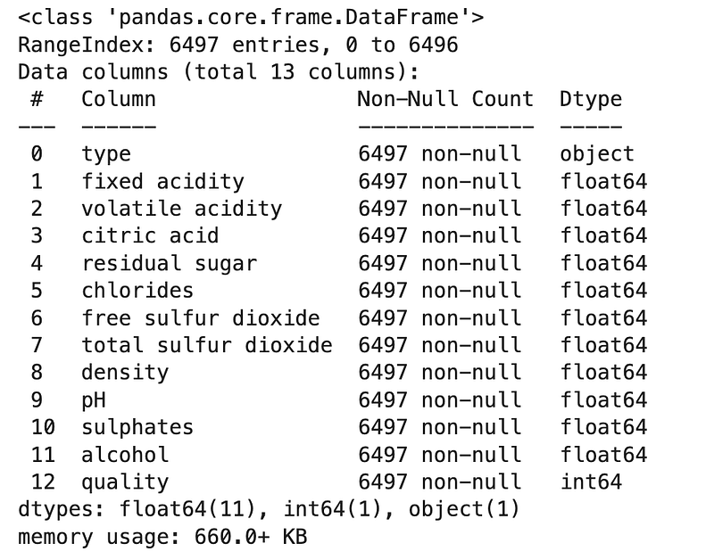

.info() is such a useful one. We can see all 13 columns (column numbers start from 0), whether there are any null values and also the data type of each of the columns.

Next, let’s look at the top 5 rows to just take a glance at a snapshot of the dataframe.

df.head()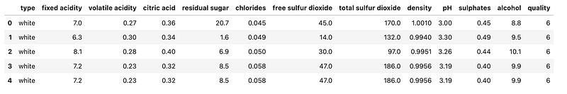

We have a couple of takeaways so far: (1) No null values; (2) float/int other than column type, which is an object.

Let’s dummy code the type column, which is the only categorical variable. Dummy coding is where the categorical variables are replaced with binary columns instead so that we have numerical variables. To better understand what dummy coding does, take a look at the column type in the results of the df.head() above. Then we will regenerate the same outputs after dummy coding for comparison.

# Dummy coding column `type`
df = pd.get_dummies(df, columns = ['type'])

Now let’s look at the columns and compare them to what we had before.

df.head()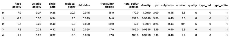

As we see in the results above, the column type is now gone and is replaced by two columns in the furthest right side named type_red and type_white. Now that we only have numerical columns, let’s proceed.

In our regression task, we will be using decision trees to predict the quality of the wine. So let’s first look at the quality column more closely.

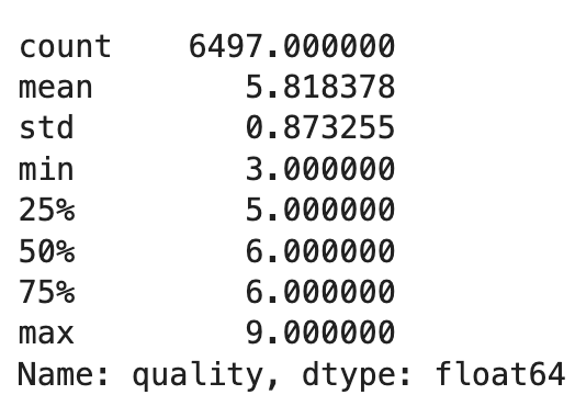
Question 1:

What are the mean and standard deviation of the quality column?

Answer:

We will use two different approaches for learning purposes.

# Approach 1
df.quality.describe()

Results:

# Approach 2
print(f"Mean is {round(df.quality.mean(), 2)} and standard deviation is {round(df.quality.std(), 2)}.")

Results:

We are going to first use decision trees as a regression model and later on will use decision trees as a classification model.

Regression vs. Classification

As discussed, decision tress can be used both for regression and classification. As a refresher:

• Regression models are used to predict a continuous output (or dependent) variable from input (or independent) variables. Some examples of such continuous output variables are quantities such as height, weight, salary, probability, etc.
• Classification models are used to predict a discrete output (or dependent) variable from input (or independent) variables (unlike regression models that predict a continuous dependent variable). We can think of each of the discrete values of the dependent variable as “classes” and hence the naming of these models. One example is the machine learning algorithm that decides whether an email is spam or not.

If you would like to learn more about regression vs. classification, visit this post.

Now that we know the distinction between regression and classification, let’s get back to our decision trees and use them for each prediction task.

2. Regression

2.1. Regression — Training

Question 2:

Split the data into train and test sets to predict the quality of the wine. For consistency, use 30% of the data as the test set and random_state of 1234.

Hint: Use sklearn.model_selection.train_test_split.

Answer:

X = df.drop('quality', axis = 1)
y = df['quality']

X_train, X_test, y_train, y_test = train_test_split(X, y, test_size = 0.3, random_state = 1234)

Question 3:

Train a decision tree regression model, using the training data. For consistency, use a max_depth of 4 for the decision tree (which is the max depth of the tree as the name suggests) and random_state of 1234.

Hint: Use sklearn.tree.DecisionTreeRegressor(). Full documentation is avaialble here.

Answer:

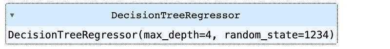
# Create an instance of the class
dtr = DecisionTreeRegressor(max_depth = 4, random_state = 1234)

# Train the model
dtr.fit(X_train, y_train)

Results:

2.2. Regression — Evaluation

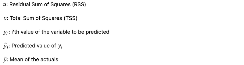
One of metrics used in evaluating the prediction of a decision tree is the coefficient of determination or R², which is defined as follows:

The best possible score is 1.0. A constant model that always predicts the expected value of y, regardless of the input features, would get R² score of 0.0.

With that knowledge, let’s look at the implementation.

Question 4:

Evaluate the trained model’s performance on the test set.

Hint: Use DecisionTreeRegressor.score().

Answer:

score_regression = dtr.score(X_test, y_test)
print(f"Coefficient of determination is {score_regression}.")

Results:

2.2.1. Evaluation through Grid Search

The score was not great. Let’s see if we can improve the model. One idea is to try different max_depth for the decision tree. sklearn.model_selection has a GridSearchCV that does this task for us.

Question 5:

Perform a grid search and see if the model score can be improved by using various tree depths. For consistency, try a depth range of 2 to 20, a random_state of 1234 and a cross-validation of 10.

Answer:

# Import grid search
from sklearn.model_selection import GridSearchCV

# Create an instance of DecisionTreeRegressor class
dtr = DecisionTreeRegressor(random_state = 1234)

# Parameters
params = {'max_depth' : [i for i in range(2, 20)]}

# Create the grid
grid = GridSearchCV(dtr, param_grid = params, cv = 10)

# Fit the model
grid.fit(X_train, y_train)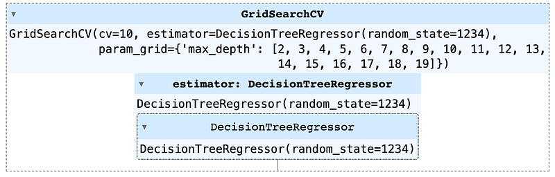

# Evaluate the model on the test set
grid.score(X_test, y_test)

Results:

The score improved some from the original attempt but the overall score is still not very high. Let’s try a different approach instead of the grid search that was explored above.

2.2.2. Evaluation through Brute Force

Brute force is when we try all the difference combinations manually. Let’s look at it in the context of an example.

Question 6:

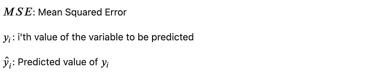
Create a loop to try various tree depths from 2 to 20 (similar to previous example) with a random_state of 1234. Then evaluate the model using the test set and create a plot that shows the depth of the tree in the X-axis and the error level in the Y-axis. For the measure of error, we can use root-mean-square error (RMSE), defined as follows:

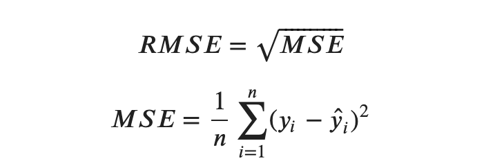
Hint: MSE can be calculated using sklearn.metrics.mean_squared_error.

Answer:

# Import mean_squared_error
from sklearn.metrics import mean_squared_error

# Create two empty lists to store errors and depths values to be used in the plot
errors = []
depths = []

for i in range(2, 20):
    # Create a dtr instance
    dtr = DecisionTreeRegressor(max_depth = i, random_state = 1234)
    
    # Fit the model to the training data
    dtr.fit(X_train, y_train)
    
    # Predict the values for the test set
    pred = dtr.predict(X_test)
    
    # Calculate RMSE
    rmse = np.sqrt(mean_squared_error(y_test, pred))
    
    # Append (add) to the errors and depths lists
    errors.append(rmse)
    depths.append(i)

Next we will plot the results.

# Create the plot
plt.figure(figsize = (14, 5))
plt.plot(depths, errors, 'o')
plt.plot(depths[errors.index(min(errors))], min(errors), 'X', markersize = 14, label = 'Lowest RMSE')

# Label the x-axix
plt.xlabel('Max Depth', fontsize = 12)

# Label the y-axix
plt.ylabel('RMSE', fontsize = 12)

# Label the plot
plt.title('Brute Force Results of the Hyperparameter Search', loc = 'center', fontsize = 15)

# Add the ticks
plt.xticks([i for i in range(2, 20)])

# Add the plot legend
plt.legend(frameon = False)
plt.show()

Results:

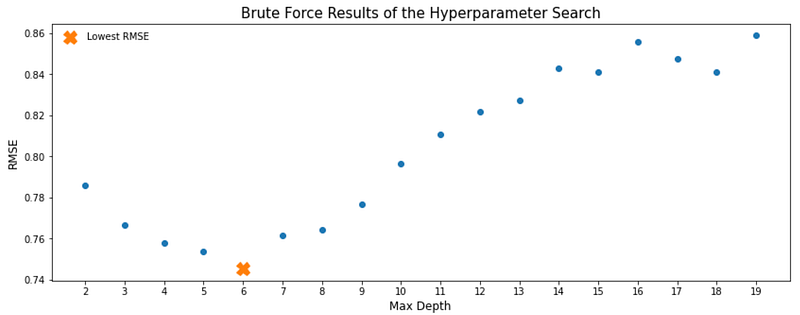
Let’s look at the plot. Lowest RMSE (which is where we want to be) happens at the max depth of 6. It is also interesting to see how RMSE changes as the max depth increases. Initially RMSE lowers as max depth increases but after the max depth of 6, RMSE also starts going up. In other words, adding to the max depth does not always result in a lower error in our model.

2.3. Regression — Feature Importance

There are various features that we used in predicting the quality of the wine in this regression exercise. In other words, each of the independent variables (all columns of the dataframe, excluding the quality column are features in our trained model). Now the next step is to find out which of these features is more important to our model. In other words, we would like to find out the predictive power of each of the features involved. This is usually referred to as “Feature Importance” in machine learning. Let’s look at an example to better understand this.

Question 7:

Which features contributed the most to this regression exercise? In other words, what are the most important features among the features used to predict the type of the wine?

Answer:

# Create an index of features
features_r = X_train.columns

# Create an array of feature importances
importances_r = dtr.feature_importances_

# Create a dataframe of feature importances
feature_importance_df_r = pd.DataFrame({'feature_names': features_r, 'feature_importance': importances_r}).sort_values('feature_importance', ascending = False)

# Show the results
feature_importance_df_r

Results:

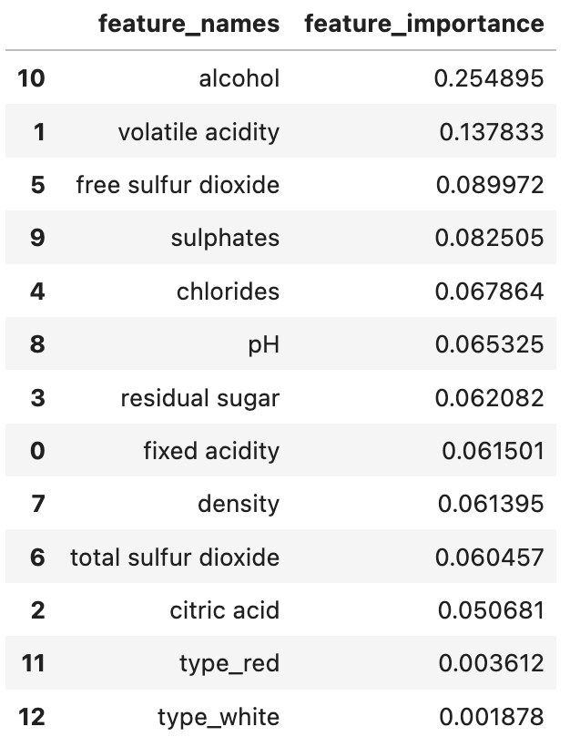
Here we can see that alcohol was the most important feature, followed by volatile acidity.

Next, we will move on from regression to classification.

3. Classification

At this stage, we are going to switch to classification and start using decision tree as a classifier. We will be trying to classify whether a wine is red or white. Therefore, let’s first read the data again and start working on our classification model.

df = pd.read_csv('wine-quality-white-and-red.csv')

And let’s look at the data as a refresher.

df.head()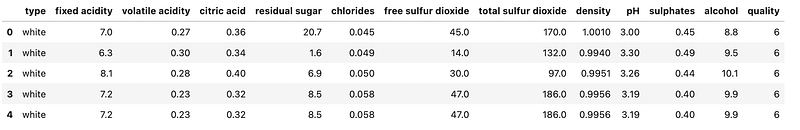

As we remember and see above, the column type is what we can use as the target variable.

Question 8:

What percentage of wines are white and what percentage are red? If the data is imbalanced, collect a random sample from the larger wine type and create a new dataframe with a balanced wine type that we can use in the next steps. For consistency, use a random_state of 1234 during downsampling.

Answer:

# Percentage of wine types
df.type.value_counts(normalize = True)

Results:

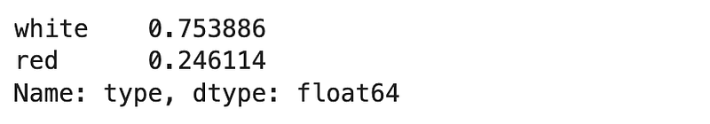
That is not balanced! We have over 75% white wines and the balance are red. Let’s also see how many each wine type is.

df['type'].value_counts()

Results:

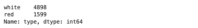
As the next step, we are going to downsample the white wines so that we will have a balanced data set of 1,599 white and 1,599 red wines as a result.

# Create a dataframe of only white wines
white_wines = df[df['type'] == 'white']

# Create a dataframe of only red wines
red_wines = df[df['type'] == 'red']

# Select a random sample from the white wines that matches the size of the red wines
white_wines_downsampled = white_wines.sample(red_wines.shape[0], random_state = 1234)

# Concatenate the two dataframes together to create our final dataframe
df_b = pd.concat([red_wines, white_wines_downsampled])

# Verify we have a balanced dataframe now
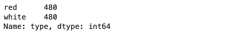
df_b.type.value_counts()

That’s perfectly balanced!

3.1. Classification — Training

Question 9:

Split the data into train and test sets to predict the type of the wine. For consistency, use 30% of the data as the test set and `random_state` of 1234.

Hint: Use sklearn.model_selection.train_test_split.

Answer:

X = df_b.drop('type', axis = 1)
y = df_b['type']

X_train, X_test, y_train, y_test = train_test_split(X, y, test_size = 0.3, random_state = 1234)

Question 10:

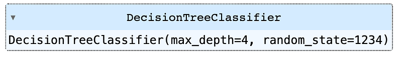
Train a decision tree classification model, using the training data. For consistency, use a max_depth of 4 for the decision tree and random_state of 1234.

Hint: Use sklearn.tree.DecisionTreeClassifier(). Full documentation is avaialble here.

Answer:

3.2. Classification — Evaluation 3.2.1. Evaluation through Accuracy

In a two-class target variable (i.e. a binary classification task) where the target variable can only be positive (or 1) and negative (or 0), there are four possible outcomes for a prediction:

• True Positive (TP): A positive event was correctly predicted.
• False Positive (FP): A negative event was incorrectly predicted as positive. This is also known as a Type I error.
• True Negative (TN): A negative event was correctly predicted.
• False Negative (FN): A positive event was incorrectly predicted as negative. This is also known as a Type II error.

Accuracy is the proportion of correct predictions over total predictions. Using the outcomes described above, we can create an equation for Accuracy as follows:

Question 11:

Evaluate the trained model’s performance (accuracy) on the test set.

Hint: Use DecisionTreeClassifier.score().

Answer:

score_classification = dtc.score(X_test, y_test)
print(f"Accuracy is {score_classification}.")

Results:

Wow! That’s an impressive accuracy but let’s make sure this is better than the weight of the population in the test set.

Question 12:

What portion of the test set is white vs. red wine?

Answer:

y_test.value_counts()

Results:

The test set, similar to the original balanced dataframe, includes equal number of red and white wines. In other words, although each class accounts for 50% of total, but the model has an accuracy of over 96%, which is quite well.

3.3. Classification — Feature Importance

Question 13:

Which features contributed the most to this classification? In other words, what are the most important features among the features used to predict the type of the wine?

Answer:

# Create an index of features
features_c = X_train.columns

# Create an array of feature importances
importances_c = dtc.feature_importances_

# Create a dataframe of feature importances
feature_importance_df_c = pd.DataFrame({'feature_names': features_c, 'feature_importance': importances_c}).sort_values('feature_importance', ascending = False)

# Show the results
feature_importance_df_c

Results:

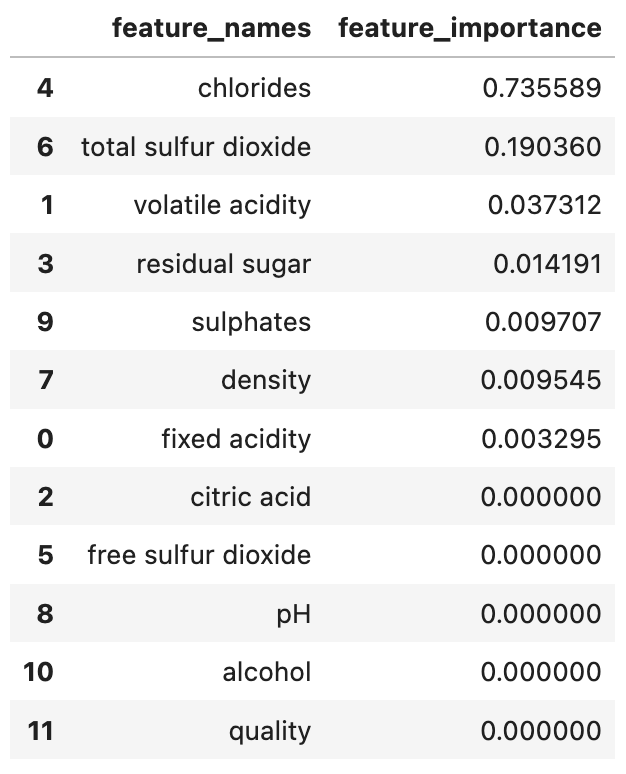
Here we can see that chlorides was the most important feature, followed by total sulfur dioxide.

4. Decision Tree Plot

Finally, we are going to visualize the performance of the classifier in a plot. I encourage you to spend a few minutes and look at different parts of the plot, after we go through this exercise. I find the exercise quite informative, in that there is so much information to grasp from a simple decision tree and it shows how powerful decision trees are in predictive regression and classification tasks.

We will be using plot_tree from skealrn.tree (documentation for reference). There are a few parameters that we will identify in this exercise so let’s go over them before diving into the exercise.

• features_names As the name suggests, this is the features used in the training process.
• class_name This one is the classes of the classification task (which was the wine type in our exercise).
• filled When set to True, paints nodes to to indicate majority class for classification.
• proportion When set to True, changes the display of values and/or samples to be proportions and percentages respectively.
• rounded When set to True, draws node boxes with rounded corners and use Helvetica fonts instead of Times-Roman.

Question 14:

Plot the decision tree associated with the classification model trained above.

Answer:

from sklearn import tree

plt.figure(figsize = (20, 10), dpi = 200)
tree.plot_tree(dtc, feature_names = features_c, class_names = y_test.unique(), filled = True, rounded = True)
plt.show()

Results:

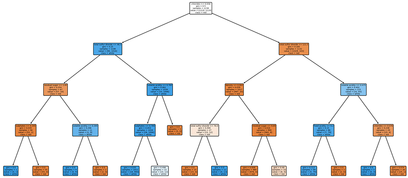
Gini importance is the same as the feature importance, which is computed as the (normalized) total reduction of the criterion brought by that feature. Gini importance is also knwon as the Mean Decrease in Impurity (MDI).

Conclusion

In this post we implemented two different tasks using decision trees, one for regression prediction and another one for a classification prediction. We started by training each of the models, then evaluating the performance of the trained models using a test set, followed by feature importance to determine the predictive power of each of the features. Lastly, we looked at how to plot decision trees, which is a visualized method of better understanding, interpreting and explaining decision trees.

Notebook with Practice Questions

Below is the notebook with both questions and answers that you can download and practice.

Thanks for Reading!

If you found this post helpful, please follow me on Medium and subscribe to receive my latest posts!