
DataRobot Auto ML for Beginners 2023 New UI
DataRobot 2023 updated Workbench version step-by-step tutorial

DataRobot is an automated machine learning platform to help users build and deploy machine learning and deep learning models quickly. This tutorial provides step-by-step instructions about how to use the new updated Workbench version released in 2023. If you do not have a DataRobot account yet, you can sign up for a 30-day free trial at https://www.datarobot.com/trial.
Resources for this post:
Let’s get started!
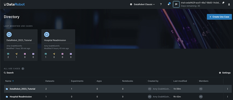
Step 1: Create a Use Case
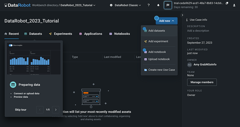
DataRobot projects are organized by use cases. After logging in DataRobot, you can click the blue Create Use Case button on the upper right corner of the page to create a new use case.

In the new use case page, you can give the use case a name. I named my use case “DataRobot_2023_Tutorial”. Then click the blue Add new button to choose an action. There are five options available, and they are:
- Add datasets
- Add experiment
- Add notebook
- Upload notebook
- Create new use case
Step 2: Add a Dataset
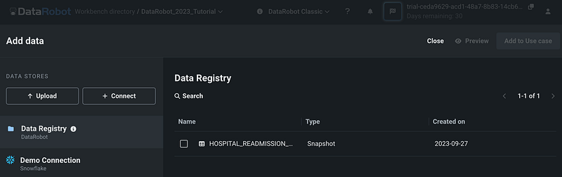
Next, let’s click Add datasets. From the Add data page, we can see that there are 3 ways to add data to a user case.
- The first way is to upload data from the local drive by clicking the Upload button.
- The second way is to read the static and snapshot datasets saved in the Data Registry.
- The third way is to read data from connected cloud platforms.
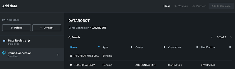
DataRobot has a Demo Connection with Snowflake, and you can see some sample schemas and tables in the demo Snowflake account.
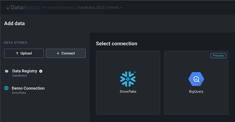
You can also create new connections with Google BigQuery or Snowflake by clicking the Connect button.
The dataset used for this tutorial is the breast cancer dataset from sklearn. You can follow this notebook to export the train and test dataset as csv files. Alternatively, you can use your own dataset to follow through the tutorial. The breast cancer dataset is for binary classification models, so using a dataset with binary labels is suggested if you would like to follow the tutorial step-by-step.
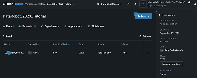
After clicking the Upload button and selecting the train_data.csv file to upload from the local drive, the uploaded data shows up in the Datasets section of the use case.
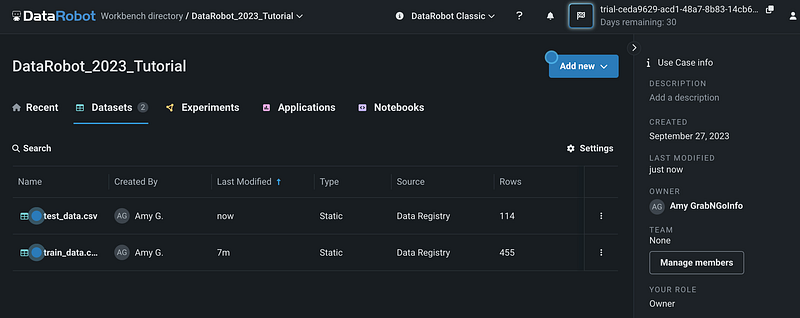
We can repeat the process to upload the test_data.csv . This dataset will be used as the data for prediction.
Step 2: Explore the Modeling Dataset
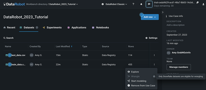
Clicking the three dots for a dataset shows the actions we can take on the dataset. We can explore the dataset, wrangle the dataset, start modeling, or remove the dataset from the use case. Currently data wrangling is only available for the Snowflake dataset.
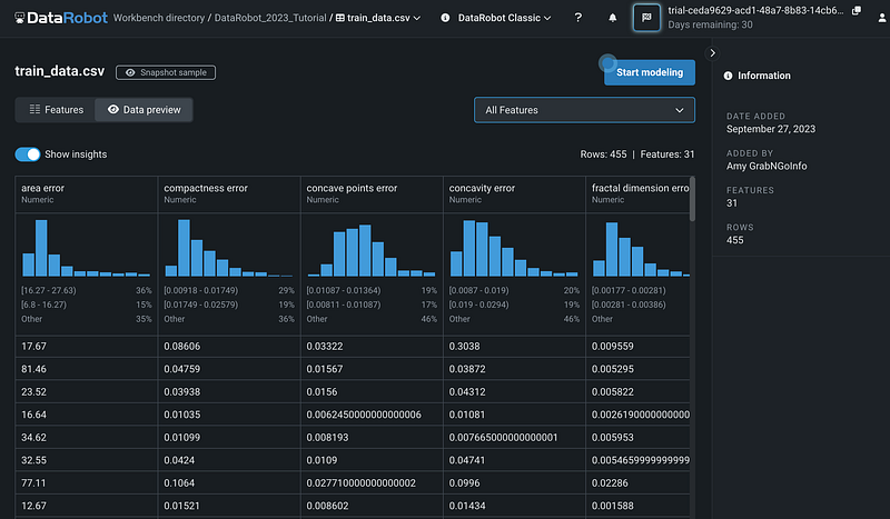
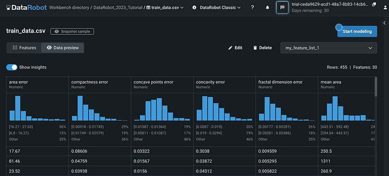
Let’s choose Explore and take a closer look at the dataset. DataRobot has two options for exploring the dataset. The Data preview shows each column in the dataset and their distributions.
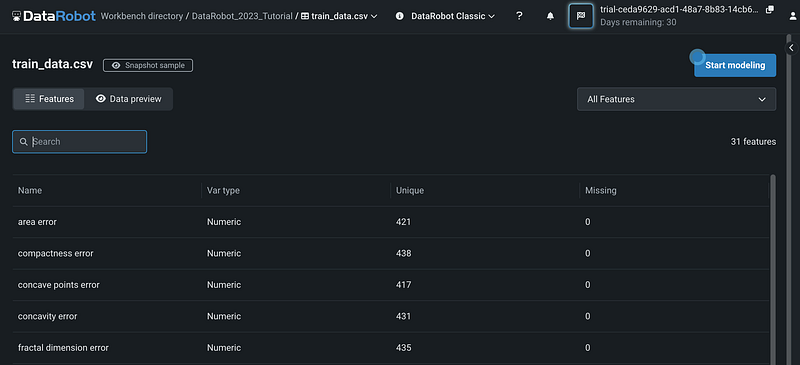
The Features view shows only the feature information, which includes feature names, variable types, the number of unique values, and the number of missing values.
Step 3: Create New Feature Lists
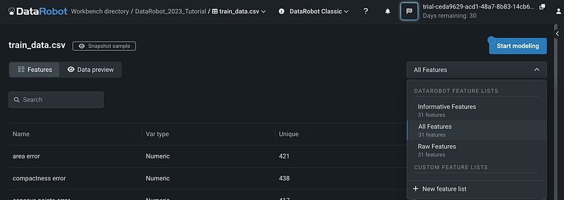
DataRobot automatically creates three feature lists. They are Informative Features, All Features, and Raw Features. We can create custom feature lists by clicking + New feature list.
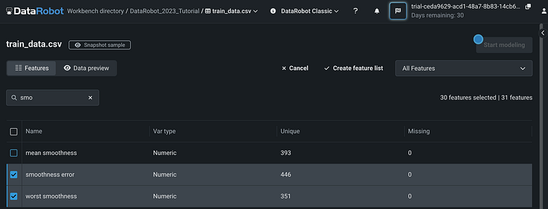
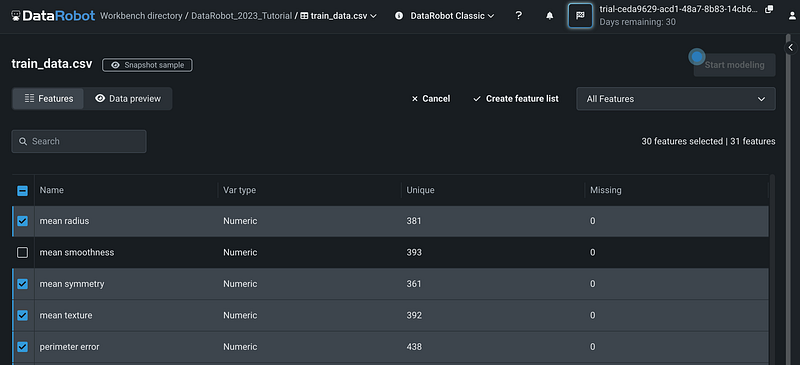
After clicking + New feature list, we can pick the features from the variable list. If most of the features are relevant and we only want to exclude a few variables, we can first select all the variables by clicking the square next to the header Name, then search the variable name to exclude, and deselect the variable. We excluded the variable mean smoothness in this example.
Next, click Create feature list to create the new custom feature list.
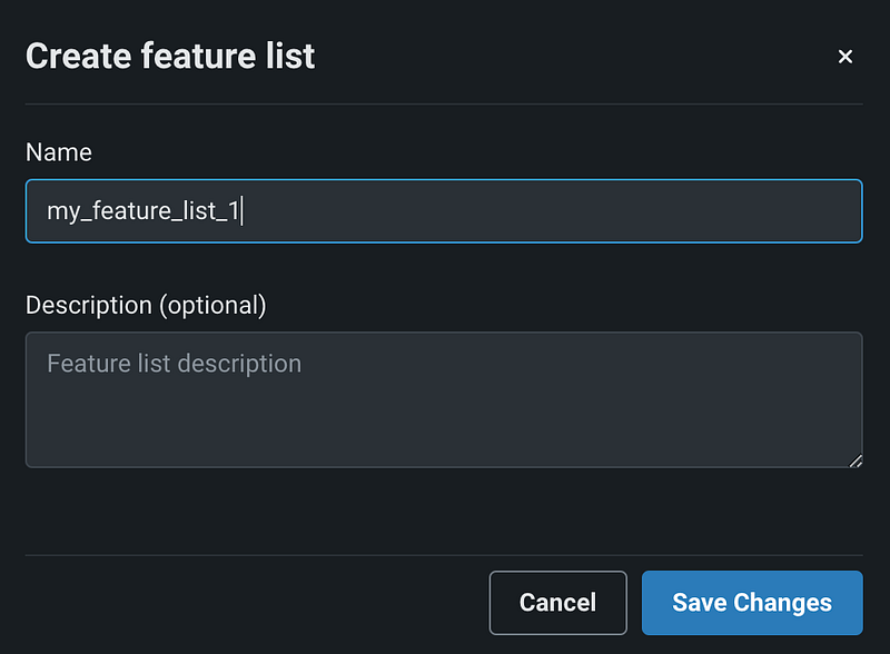
A new window pops up for us to enter the name of the feature list. I gave it the name of my_feature_list_1. We can also enter the optional description for the feature list. Click the blue Save Changes button to save the feature list.
Step 4: Start Modeling
After finishing creating the custom feature list, click the blue Start modeling button to start the modeling process.
Step 5: Select Target Variable and Feature List
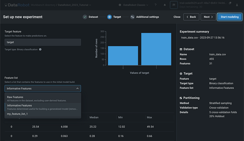
Enter the target feature name under the section Target feature, and a bar chart about the target variables distribution will be automatically created.
Under Feature list, select the feature list that you would like to use to build the model.
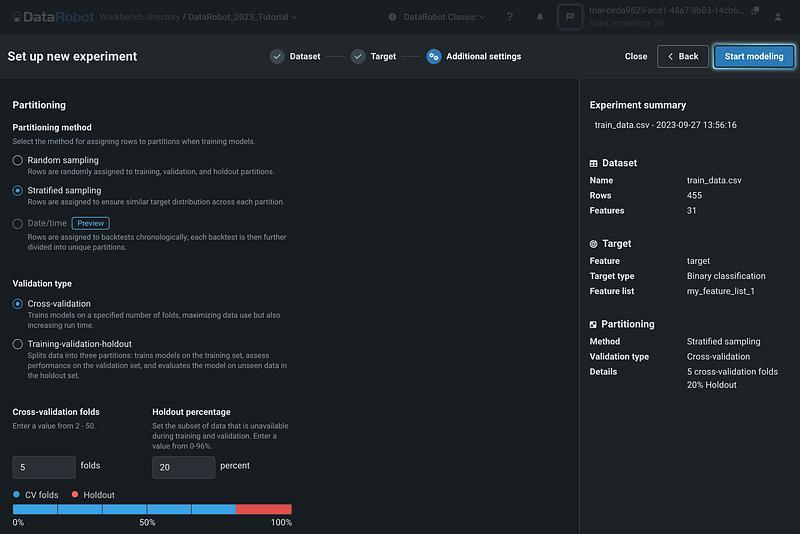
You can click Next to open the Additional Settings page, where you can change the partitioning method, validation type, as well as holdout percentage.
Step 6: Build Models
Next, click the blue Start Modeling button to start building the models.
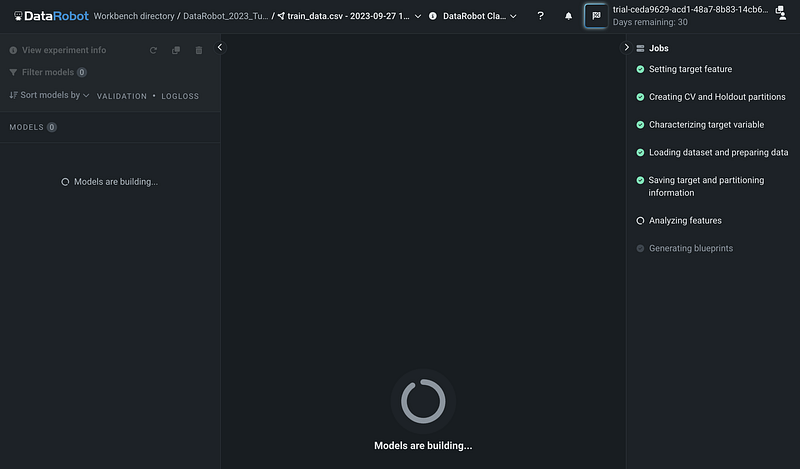
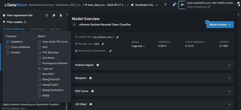
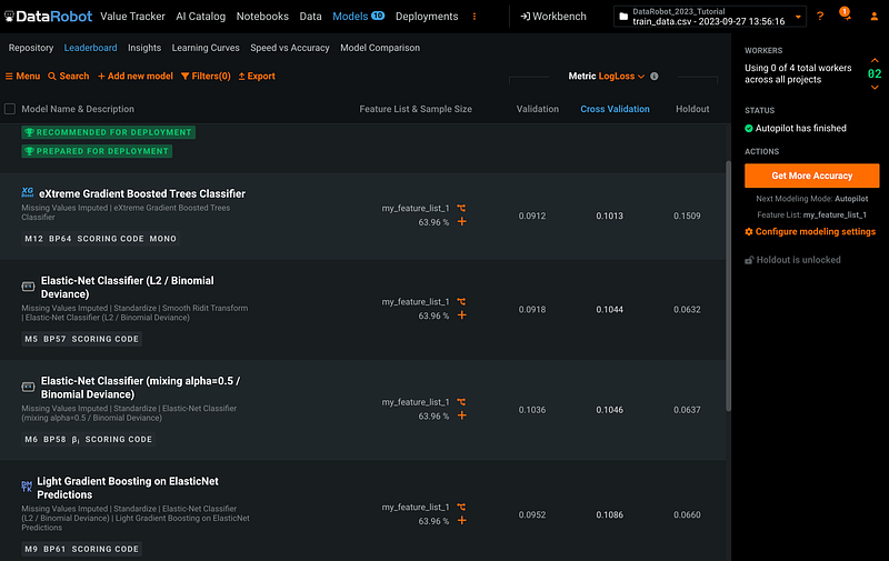
DataRobot automatically builds a few models and ranks the models based on the performance metric. The default metric is log loss for the validation dataset, but we can click the Sort models by button to make changes.
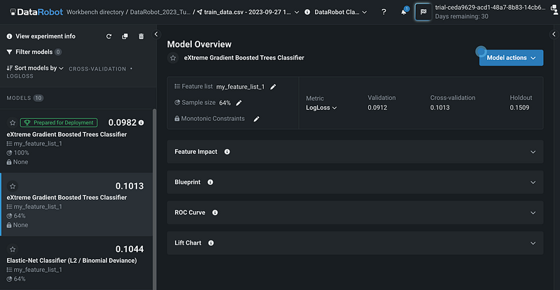
I changed the partition from Validation to Cross-validation, and the models are re-ranked based on the cross-validation log loss values.
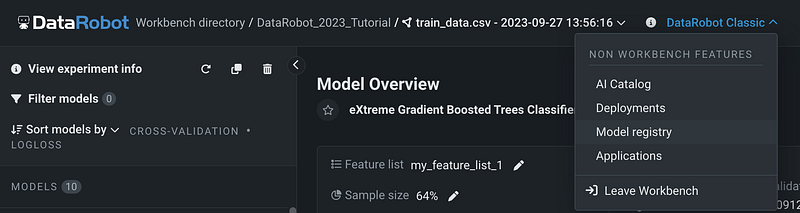
Step 7: Switch to DataRobot Classic
To get access to other model algorithms, we need to switch to DataRobot Classic.
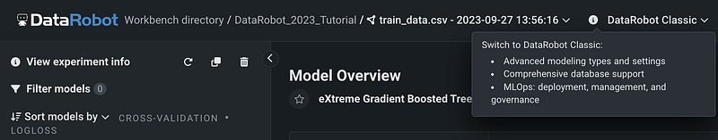
Click DataRobot Classic and select Model Registry.
You will switch from Workbench to DataRobot Classic. Now select Models, and you will see the 10 models built in the Workbench.
We can switch back to Workbench by clicking the Workbench button.
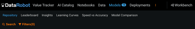
Step 8: Search New Model Algorithms
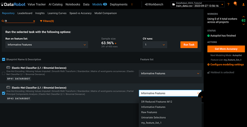
To search new model algorithms, click Repository under Models, then click the orange Search.
In the search bar, enter the keyword for the model algorithm. In this example, I am searching L1, and get two L1 models as the search results.
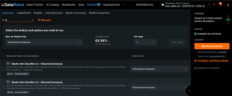
Step 9: Add New Model Algorithms
Click the square next to the model you want to use and select the feature list for the model. In this example, I selected model number BP43 and the custom feature list my_feature_list_1. Click the orange Run Task button to run the task.
Step 10: Switch Back to WorkBench
After the model is completed, you can continue with the DataRobot Classic or go back to the Workbench. We will go back to Workbench by clicking the Workbech button. To learn how to evaluate the model performance using DataRobot Classic, please refer to my previous tutorial.
After returning the Workbench, select the DataRobot_2023_Tutorial use case.
Then click Experiments. We can see that we have 1 experiment with 11 models.
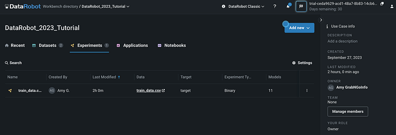
Clicking on the experiment opens up the details for the 11 models.
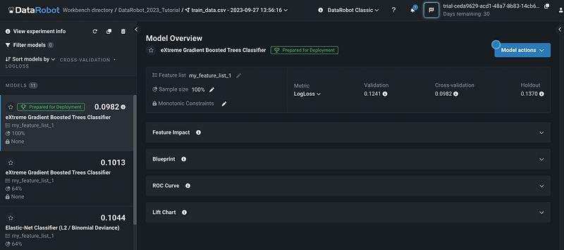
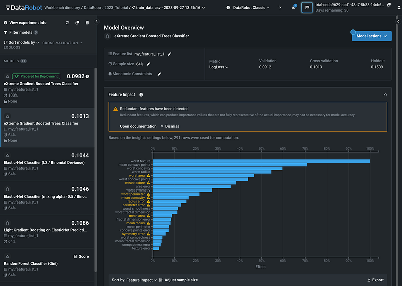
Step 11: Feature Importance
Click a model on the left pane to select the model, then click Feature Impact. DataRobot highlighted the features that have high correlations with other features.
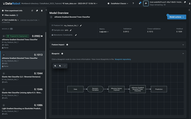
Step 12: Blueprint
The Blueprint of the model shows the general workflow for building the model.
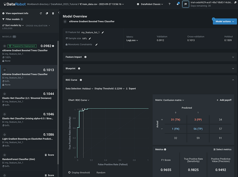
Step 13: Model Performance Metrics
The ROC Curve section has the ROC chart, the confusion matrix, and other important model metrics such as Precision, Recall, and F1 score.
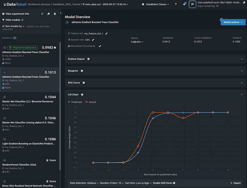
Step 14: Lift Chart
The Lift Chart section has a graph with Bins based on the predicted value on the x-axis, and the average target value on the y-axis. Both the predicted and the actual values are plotted.
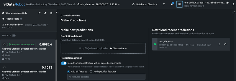
Step 15: Make Predictions
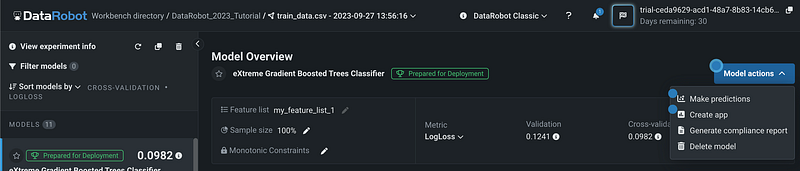
Let’s use the XGBoost model with the best performance to make predictions. Select the model and click the blue Model Action button, then select Make Predictions.
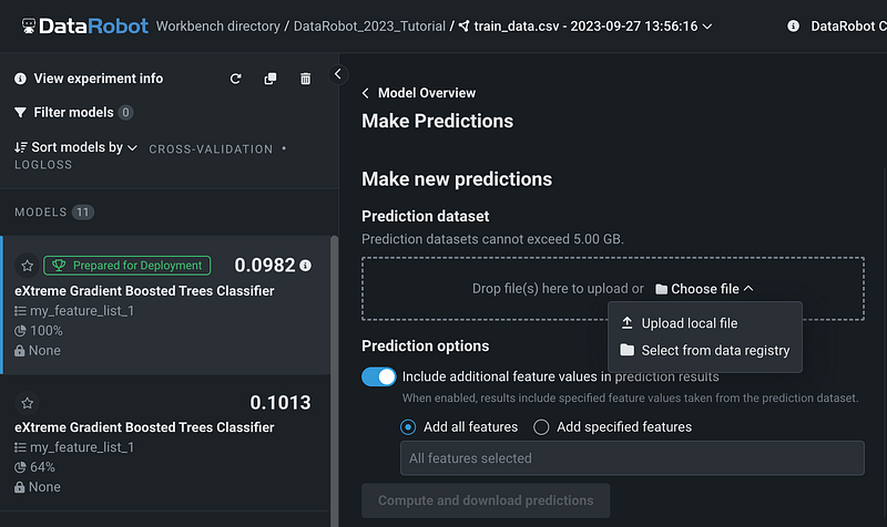
We can drop the prediction dataset, upload a file from the local drive, or select from the data registry. Because we already uploaded the prediction dataset to the data registry, we will select from the data registry.
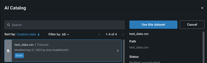
Let’s select test_data.csv and click the blue Use this dataset button.
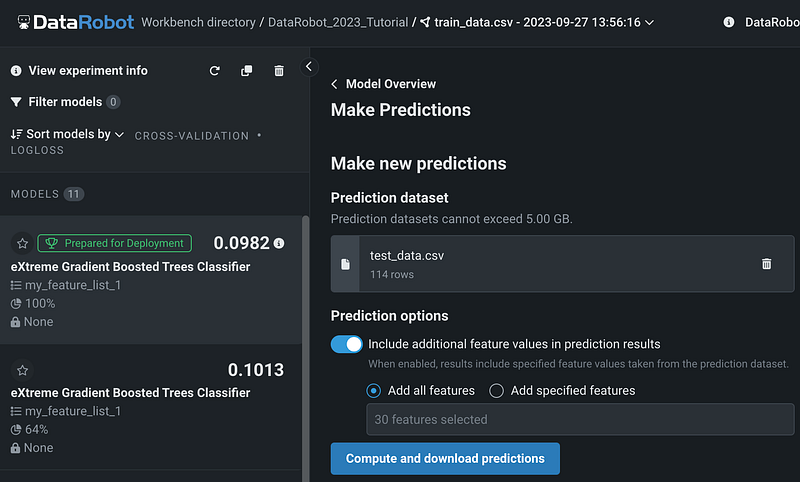
We can choose to include feature values in prediction results by keeping the Prediction options on, then click Compute and download predictions.
Step 16: Download Predictions
After the prediction is completed, it’s available to download for 48 hours.
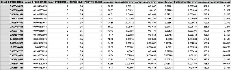
The prediction results have the predicted probabilities and the predicted labels for both the positive class and the negative class, as well as all the feature values.
More tutorials are available on GrabNGoInfo YouTube Channel and GrabNGoInfo.com
Recommended Tutorials
- GrabNGoInfo Machine Learning Tutorials Inventory
- Data Science Project Completed in 5 Minutes Using ChatGPT Plugin Noteable
- Recommendation System: User-Based Collaborative Filtering
- Recommendation System: Item-Based Collaborative Filtering
- Topic Modeling with Deep Learning Using Python BERTopic
- Five Ways To Create Tables In Databricks
- Hyperparameter Tuning for Time Series Causal Impact Analysis in Python
- Top 20 AB Test Interview Questions and Answers
- Top 10 Causal Inference Interview Questions and Answers


