Databricks MLflow Tracking For Linear Regression Model

How to use MLflow to track different model versions and retrieve experiment information?

MLflow is an open-source platform for machine learning lifecycle management. MLflow on Databricks offers an integrated experience for running, tracking, and serving machine learning models. In this tutorial, we will cover:

How to use MLflow to track different model versions?
How to retrieve MLflow experiment information programmatically?
How to retrieve MLflow information using Databricks UI?

Resources for this post:

Video tutorial for this post on YouTube
Databricks notebook with code
More video tutorials on Databricks and PySpark
More blog posts on Databricks and PySpark

Let’s get started!

Step 1: Import Libraries

In step 1, we will import the libraries. pandas, numpy, and pyspark SQL functions are for data processing.

matplotlib is for visualization.

make_regression is for creating synthetic modeling datasets.

From the pyspark.ml library, we imported VectorAssembler for feature formatting, LinearRegression for model training, RegressionEvaluator for model evaluation, and Pipeline for pipeline creation and loading.

We also imported mlflow, mlflow.spark for the spark flavor, and MlflowClient to query model information. If you are using the Databricks runtime for machine learning, MLflow is installed. Otherwise, the MLflow package can be installed from PyPI.

# Data processing
import pandas as pd
import numpy as np
from pyspark.sql.functions import log, col, exp

# Visulaization
import matplotlib.pyplot as plt

# Create synthetic dataset
from sklearn.datasets import make_regression

# Modeling
from pyspark.ml.feature import VectorAssembler
from pyspark.ml.regression import LinearRegression
from pyspark.ml.evaluation import RegressionEvaluator
from pyspark.ml import Pipeline

# MLflow
import mlflow
import mlflow.spark
from mlflow.tracking import MlflowClient

Join Medium with my referral link - Amy @GrabNGoInfo

Read every story from Amy (and thousands of other writers on Medium). Your membership fee directly supports Amy and…

medium.com

Step 2: Create Dataset For Linear Regression

In step 2, we will create a synthetic dataset for the linear regression model.

Using make_regression, a dataset with one million records is created. The dataset has two features, and both of them are informative. It has a noise of 10 and a bias of 2. random_state ensures the randomly created dataset is reproducible. The random state does not have to be 42. It can be any number.

# Create a synthetic dataset
X, y = make_regression(n_samples=1000000, 
                       n_features=2, 
                       n_informative=2,
                       noise=10, 
                       bias=2, 
                       random_state=42)

After the dataset is created, we can scale the values to the desired ranges. In this example, the first feature is scaled to values between 1 and 100, the second feature is scaled to values 1000 and 5000, and the target is scaled to values between 3000 and 80,000.

# Scale feature 1 to values between 1 and 100
X[:, 0] = np.interp(X[:, 0], (X[:, 0].min(), X[:, 0].max()), (1, 100))

# Scale feature 2 to values between 1000 and 5000
X[:, 1] = np.interp(X[:, 1], (X[:, 1].min(), X[:, 1].max()), (1000, 5000))

# Scale dependent variable to values between 3000 and 80000
y = np.interp(y, (y.min(), y.max()), (3000, 80000))

The output of make_regression is in array format. We convert it into a pandas dataframe, then the pandas dataframe is converted into a spark dataframe.

# Convert the data from numpy array to a pandas dataframe
pdf = pd.DataFrame({'feature1': X[:, 0], 'feature2': X[:, 1], 'dependent_variable': y})

# Convert pandas dataframe to spark dataframe
sdf = spark.createDataFrame(pdf)

# Check data summary statistics
display(sdf.summary())

summary() gives us the summary statistics of the dataset.

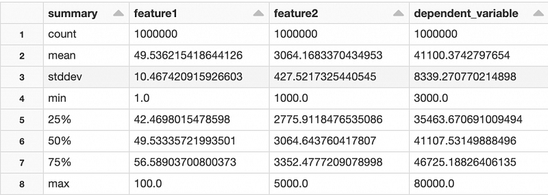
Synthetic Data For Linear Regression — Image from GrabNGoInfo.com

Next, let’s check the scatterplot between the features and the dependent variable. The visualization was created using the Databricks notebook built-in functionality. To learn more about it, please check out my previous tutorial on Databricks Dashboard For Big Data.

display(sdf.select('dependent_variable', 'feature1'))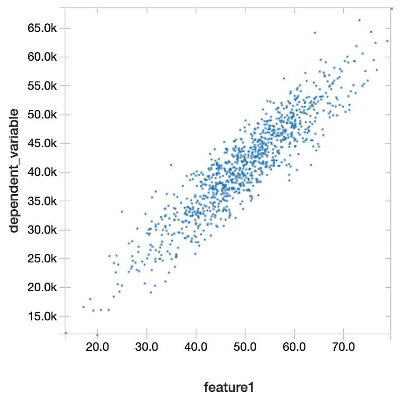

Scatterplot between the feature1 and the dependent variable — Image from GrabNGoInfo.com

display(sdf.select('dependent_variable', 'feature2'))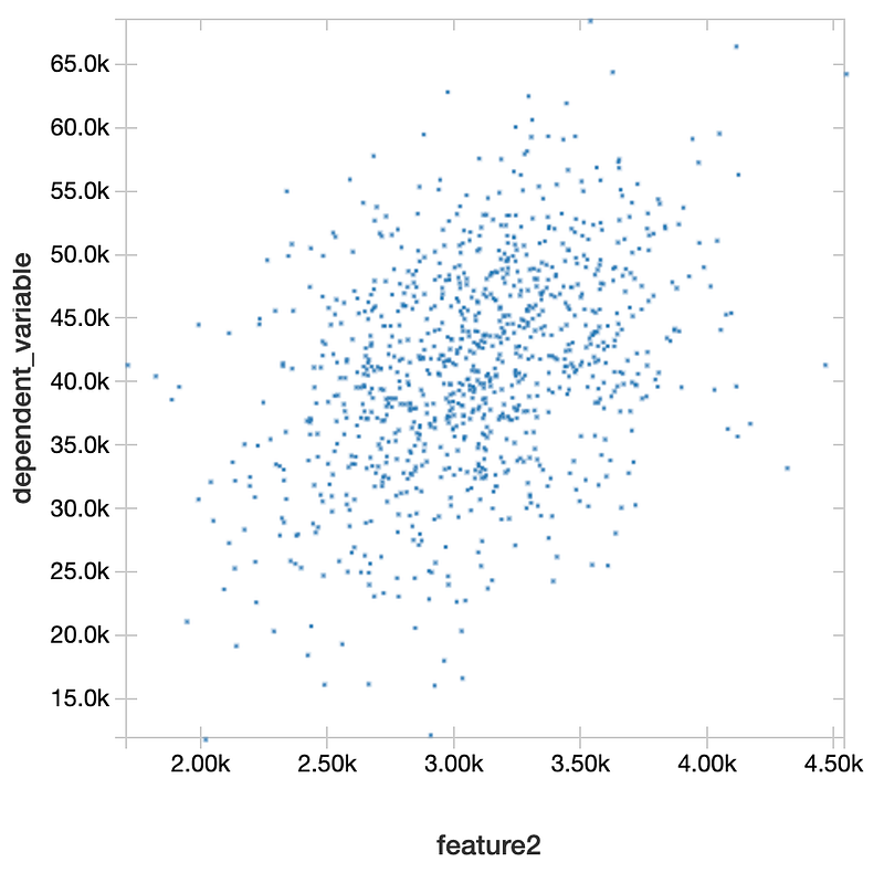

Scatterplot between the feature2 and the dependent variable — Image from GrabNGoInfo.com

We can see that both features’ scatterplots show positive trends, but their shape and slope are different.

Step 3: Train Test Split

After creating the modeling dataset, in step 3, we will make the train test split.

Using randomSplit, we split the dataset into 80% training and 20% validation. seed=42 makes the random split results reproducible. However, we need to make sure that the same cluster and partition number are used when reproducing the split.

We got 800,299 in the training dataset and 199,701 in the testing dataset after the split.

# Train test split
trainDF, testDF = sdf.randomSplit([.8, .2], seed=42)

# Print the number of records
print(f'There are {trainDF.cache().count()} records in the training dataset.')
print(f'There are {testDF.cache().count()} records in the testing dataset.')

Step 4: Linear Regression With Raw Data — Model 1

In step 4, we will create the first model using linear regression. In this model, the features and the dependent variable created in the synthetic dataset will be used directly. So let’s give it the run name of LR-Raw-Data.

Firstly, a linear regression model is trained using spark ML. To learn more details, please check out my previous tutorial on Databricks Linear Regression With Spark ML.

Then the parameter of the model is logged. For this experiment, we plan to create two versions of the model, one with the raw dependent variable, and the other with the logarithm of the dependent variable. Model 1 uses the raw dependent variable. To log this information, we saved the name of the dependent variable into a parameter called target_variable.

We also logged the parameter for the elastic net. 0.5 means 50% of LASSO (L1) regularization and 50% of Ridge (L2) regularization. To learn more about regularization, please check out my previous tutorial on LASSO (L1) Vs Ridge (L2) Vs Elastic Net Regularization.

After that, we logged the model for this run, made predictions on the testing dataset, and saved the prediction CSV file as an artifact.

When doing model performance evaluation, we calculated RMSE, R Square, MSE, and MAE. And they are logged as the experiment metrics.

Finally, a plot for the dependent variable distribution is created and logged as an artifact.

with mlflow.start_run(run_name="LR-Raw-Data") as run:
    # Define pipeline
    vecAssembler = VectorAssembler(inputCols=["feature1", "feature2"], outputCol="features")
    lr = LinearRegression(featuresCol="features", labelCol="dependent_variable", predictionCol="prediction",elasticNetParam=0.5)
    pipeline = Pipeline(stages=[vecAssembler, lr])
    pipelineModel = pipeline.fit(trainDF)

    # Log parameters
    mlflow.log_param("target_variable", "dependent_variable")
    mlflow.log_param("elasticNetParam", 0.5)

    # Log the model for this run
    mlflow.spark.log_model(pipelineModel, "SparkML-linear-regression")

    # Make predictions
    predDF = pipelineModel.transform(testDF)    
    
    # Save the prediction as csv
    predDF.toPandas().to_csv('predictions.csv', index=False)
    
    # Log the saved prediction as artifact
    mlflow.log_artifact("predictions.csv")
    
    # Evaluate predictions
    regressionEvaluator = RegressionEvaluator(predictionCol="prediction", labelCol="dependent_variable")
    rmse = regressionEvaluator.setMetricName("rmse").evaluate(predDF)
    r2 = regressionEvaluator.setMetricName("r2").evaluate(predDF)
    mse = regressionEvaluator.setMetricName("mse").evaluate(predDF)
    mae = regressionEvaluator.setMetricName("mae").evaluate(predDF)
    
    # Log metrics
    mlflow.log_metric("rmse", rmse)
    mlflow.log_metric("r2", r2)    
    mlflow.log_metric("mse", mse)    
    mlflow.log_metric("mae", mae)

    # Create a plot for the testing dataset
    testDF.toPandas().hist(column="dependent_variable", bins=100)
    
    # Log artifact
    plt.savefig("dependent_variable.png")
    mlflow.log_artifact("dependent_variable.png")

Step 5: Linear Regression With Log Target — Model 2

Taking logarithm is a commonly used technique for data transformation. It is usually used to transform non-normal distributed data into a normal distribution. Our synthetic data is already normally distributed, so it does not need the logarithm. But we would like to create a model version with log transformation for illustration purposes.

Firstly, we name the run LR-Log-Target, indicating that the target variable is the logarithm transformation of the raw data.

Then the logarithm of the dependent variable is created for both the training dataset and the testing dataset.

The rest of the code is very similar to the previous model, except for three changes. The first change is the information related to the dependent variable is updated to the logarithm version. The second change is that the elasticNetParam is changed from 0.5 to 0.8. The third change is related to the model prediction. Because the target label for the model training is in logarithm form, the predicted values are in logarithm too. So we need to take the exponential of the predictions before doing a model performance evaluation.

with mlflow.start_run(run_name="LR-Log-Target") as run:
    # Take the log of the target variable
    logTrainDF = trainDF.withColumn("log_dv", log(col("dependent_variable")))
    logTestDF = testDF.withColumn("log_dv", log(col("dependent_variable")))

    # Define pipeline
    vecAssembler = VectorAssembler(inputCols=["feature1", "feature2"], outputCol="features")
    lr = LinearRegression(featuresCol="features", labelCol="log_dv", predictionCol="log_prediction", elasticNetParam=0.8)
    pipeline = Pipeline(stages=[vecAssembler, lr])
    pipelineModel = pipeline.fit(logTrainDF)

    # Log parameters
    mlflow.log_param("target_variable", "log_dv")
    mlflow.log_param("elasticNetParam", 0.8)

    # Log model
    mlflow.spark.log_model(pipelineModel, "SparkML-linear-regression")

    # Make predictions
    predDF = pipelineModel.transform(logTestDF)
    expDF = predDF.withColumn("prediction", exp(col("log_prediction")))
    
    # Save the prediction as csv
    predDF.toPandas().to_csv('predictions.csv', index=False)
    
    # Log the samved prediction as artifact
    mlflow.log_artifact("predictions.csv")
    
    # Evaluate predictions
    regressionEvaluator = RegressionEvaluator(predictionCol="prediction", labelCol="dependent_variable")
    rmse = regressionEvaluator.setMetricName("rmse").evaluate(expDF)
    r2 = regressionEvaluator.setMetricName("r2").evaluate(expDF)
    mse = regressionEvaluator.setMetricName("mse").evaluate(expDF)
    mae = regressionEvaluator.setMetricName("mae").evaluate(expDF)
    
    # Log metrics
    mlflow.log_metric("rmse", rmse)
    mlflow.log_metric("r2", r2)    
    mlflow.log_metric("mse", mse)    
    mlflow.log_metric("mae", mae)    
    
    # Create a plot for the testing dataset
    logTestDF.toPandas().hist(column="log_dv", bins=100)
    
    # Log artifact
    figPath = 'grabngoinfo_' + "logDv.png" 
    plt.savefig("log_dependent_variable.png")
    mlflow.log_artifact("log_dependent_variable.png")

Step 6: Get Model Experiments Information Programmatically

In step 6, we will get model experiment information programmatically.

list_experiments() from MlflowClient() lists all the experiments and their IDs.

# List MLflow experiments
MlflowClient().list_experiments()

There are two types of experiments, workspace experiments and notebook experiments.

Workspace experiments are created from the Databricks Machine Learning UI or the MLflow API. Any notebook can log runs to a workspace experiment by experiment ID or experiment name. We can access a workspace experiment from the workspace menu.
Notebook experiments are associated with specific notebooks. The experiment is automatically created by Databricks. We can access a notebook experiment from the notebook.

The experiment in this tutorial is a notebook experiment.

To get all the runs for an experiment, use mlflow.search_runs and pass in the experiment_id.

# Get all runs for a given experiment
experiment_id = run.info.experiment_id
runs_df = mlflow.search_runs(experiment_id)

# Display information
runs_df.T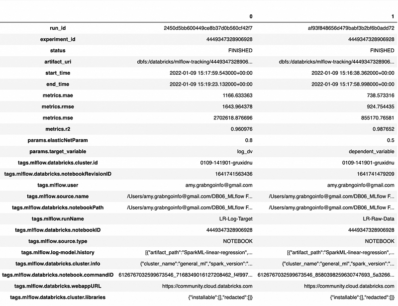

Databricks getting all the runs for an MLflow experiment — Image from GrabNGoInfoc.om

We can see that the model with the raw data has better performance than the log version of the data.

When there are a lot of runs in an experiment, we may want to sort the runs in descending time order and get the information for the latest runs. max_results controls the number of runs to keep.

# Get the the latest run
runs = MlflowClient().search_runs(experiment_id, order_by=["attributes.start_time desc"], max_results=1)

# Get the metrics from the latest run
runs[0].data.metrics

Output

Out[33]: {'mae': 1166.6333634351645,
 'mse': 2702618.876696308,
 'r2': 0.9609755978839164,
 'rmse': 1643.9643781713485}

Step 7: Get Model Experiments Information Using UI

In step 7, we will talk about how to use Databricks UI to retrieve the experiment information.

Step 7.1: Access the experiment information within a notebook

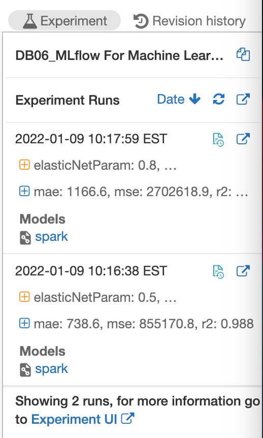
To access the experiment information within the notebook, we can click the Experiment icon on the upper right of the notebook. The two versions of the models are shown on the right sidebar of the notebook.

Access the experiment information within a Databricks notebook — Image from GrabNGoInfo.com

Step 7.2: Access Experiment UI

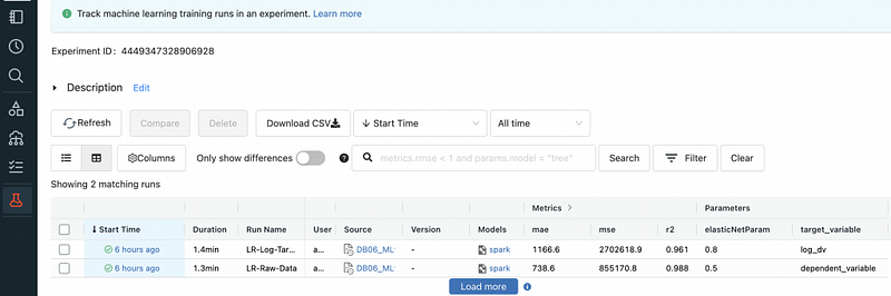
To open the full experiment UI on a new page, click the blue Experiment UI at the bottom of the sidebar.

Step 7.3: Access Experiment Run Information

To check the details of a run, click either the blue Start Time (6 hours ago in this example) or the blue spark under Models for the run.

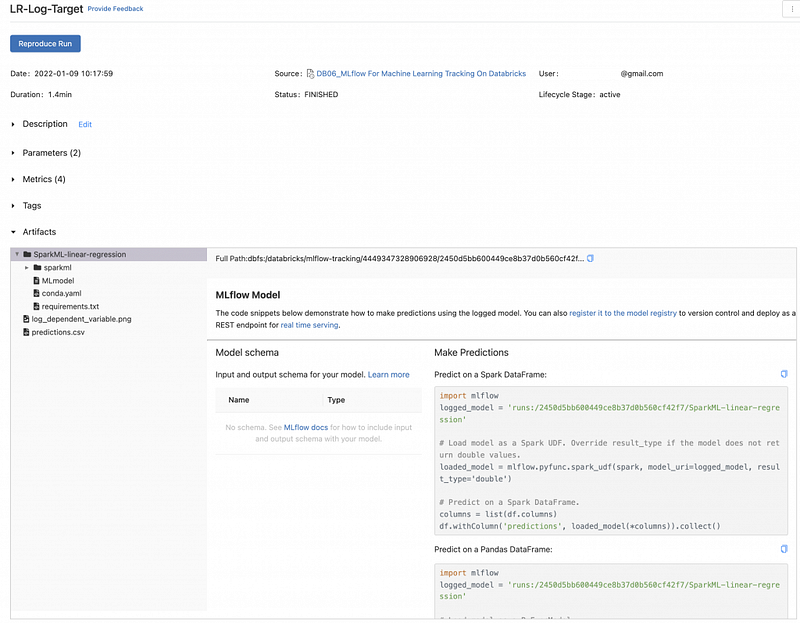
Databricks MLflow Experiment Run UI — Image from GrabNGoInfo.com

We can get detailed information about this run by clicking the list of options on the left-hand side of the UI. It also provides the code for prediction using Spark and pandas dataframe.

Summary

In this tutorial, we talked about how to use MLflow to track the spark ML linear regression models. We covered:

How to use MLflow to track different model versions?
How to retrieve MLflow experiment information programmatically?
How to retrieve MLflow information using Databricks UI?

More tutorials are available on GrabNGoInfo YouTube Channel and GrabNGoInfo.com.

Recommended For You

References

Join Medium with my referral link - Amy GrabNGoInfo

As a Medium member, a portion of your membership fee goes to writers you read, and you get full access to every story…

medium.com