
LASSO (L1) Vs Ridge (L2) Vs Elastic Net Regularization For Classification Model
Choosing among LASSO, Ridge, and Elastic Net Regularization by comparing their performances

LASSO (Least Absolute Shrinkage and Selection Operator) is also called L1 regularization, and Ridge is also called L2 regularization. Elastic Net is the combination of LASSO and Ridge. All three are techniques commonly used in machine learning to correct overfitting.
In this tutorial, we will cover
- What’s the difference between LASSO (L1), Ridge (L2), and Elastic Net?
- How to run LASSO for classification model using Python
sklearn? - How to run Ridge for the classification model?
- How to run Elastic Net for the classification model?
- How to compare the performance of LASSO, Ridge, and Elastic Net?
Resources for this post:
- Video tutorial on YouTube
- Python code is at the end of the post. Click here for the notebook.
- More video tutorials on Overfitting Correction
- More blog posts on Overfitting Correction
Let’s get started!
Step 0: LASSO (L1) vs Ridge (L2) vs. Elastic Net
In step 0, we will talk about the differences between LASSO, Ridge, and elastic net.
LASSO and Ridge regularization correct overfitting by shrinking the coefficient of the model. During the model training process, instead of minimizing the model training error, they minimize the model training error plus a penalty term. LASSO and Ridge have different calculation algorithms for the penalty term. Elastic net’s penalty term is a combination of the algorithm from LASSO and Ridge.
- The penalty term has a parameter called lambda. It controls the strength of the penalty.
When lambda equals 0, the penalty term equals 0. So the model is a model with no regularization.
When lambda increases, the penalty term value increases, and the model coefficients values decrease.
When lambda goes infinity, the model coefficients shrink to nearly 0. The model is left with only the intercept, which predicts the average value for every data point.
- LASSO’s penalty term is the penalty parameter lambda multiplied by the sum of the absolute value of the coefficients. Because LASSO’s coefficients may shrink to zeros, it can be used for automatic feature selection.
- Ridge shrinks the model coefficients based on the sum of the squared coefficients. Ridge does not shrink the model coefficients to zero.
- Elastic net’s penalty term is a combination of LASSO and Ridge regression’s penalty term. It sets some coefficients to zeros, but the number is smaller than LASSO.
Step 1: Import Libraries
In the first step, let’s import the Python libraries needed for this tutorial.
We will use the breast cancer dataset for this tutorial, so datasets from sklearn needs to be imported. pandas and numpy are imported for data processing. matplotlib is for visualization, and StandardScaler is for data standardization.
For model training, we imported train_test_split and LogisticRegression.
For model performance evaluation, we imported plot_confusion_matrix, classification_report, log_loss, roc_curve, and roc_auc_score.
# Dataset
from sklearn import datasets
# Data processing
import pandas as pd
import numpy as np# Visualization
import matplotlib.pyplot as plt# Standardize the data
from sklearn.preprocessing import StandardScaler# Model and performance evaluation
from sklearn.model_selection import train_test_split
from sklearn.linear_model import LogisticRegression
from sklearn.metrics import plot_confusion_matrix, classification_report, log_loss, roc_curve, roc_auc_scoreStep 2: Read In Data
In the second step, the breast cancer data from sklearn library is loaded and transformed into a pandas dataframe.
# Load the breast cancer dataset
data = datasets.load_breast_cancer()
# Put the data in pandas dataframe format
df = pd.DataFrame(data=data.data, columns=data.feature_names)
df['target']=data.target# Check the data information
df.info()The information summary shows that the dataset has 569 records and 31 columns.
<class 'pandas.core.frame.DataFrame'>
RangeIndex: 569 entries, 0 to 568
Data columns (total 31 columns):
 #   Column                   Non-Null Count  Dtype
---  ------                   --------------  -----
 0   mean radius              569 non-null    float64
 1   mean texture             569 non-null    float64
 2   mean perimeter           569 non-null    float64
 3   mean area                569 non-null    float64
 4   mean smoothness          569 non-null    float64
 5   mean compactness         569 non-null    float64
 6   mean concavity           569 non-null    float64
 7   mean concave points      569 non-null    float64
 8   mean symmetry            569 non-null    float64
 9   mean fractal dimension   569 non-null    float64
 10  radius error             569 non-null    float64
 11  texture error            569 non-null    float64
 12  perimeter error          569 non-null    float64
 13  area error               569 non-null    float64
 14  smoothness error         569 non-null    float64
 15  compactness error        569 non-null    float64
 16  concavity error          569 non-null    float64
 17  concave points error     569 non-null    float64
 18  symmetry error           569 non-null    float64
 19  fractal dimension error  569 non-null    float64
 20  worst radius             569 non-null    float64
 21  worst texture            569 non-null    float64
 22  worst perimeter          569 non-null    float64
 23  worst area               569 non-null    float64
 24  worst smoothness         569 non-null    float64
 25  worst compactness        569 non-null    float64
 26  worst concavity          569 non-null    float64
 27  worst concave points     569 non-null    float64
 28  worst symmetry           569 non-null    float64
 29  worst fractal dimension  569 non-null    float64
 30  target                   569 non-null    int64
dtypes: float64(30), int64(1)
memory usage: 137.9 KB
The target variable distribution shows 63% of ones and 37% of zeros in the dataset. Therefore, one means the patient has breast cancer, and 0 represents the patient does not have breast cancer.
# Check the target value distribution
df['target'].value_counts(normalize=True)
1 0.627417
0 0.372583
Name: target, dtype: float64Step 3: Train Test Split
In step 3, we split the dataset into 80% training and 20% testing dataset. random_state makes the random split results reproducible.
# Train test split
X_train, X_test, y_train, y_test = train_test_split(df[df.columns.difference(['target'])], df['target'], test_size=0.2, random_state=42)
# Check the number of records in training and testing dataset.
print(f'The training dataset has {len(X_train)} records.')
print(f'The testing dataset has {len(X_test)} records.')The training dataset has 455 records, and the testing dataset has 114 records.
The training dataset has 455 records.
The testing dataset has 114 records.
Step 4: Standardization
Standardization is to rescale the features to the same scale. It is calculated by extracting the mean and divided by the standard deviation. After standardization, each feature has zero mean and unit standard deviation.
Standardization should be fit on the training dataset only to prevent test dataset information from leaking into the training process. Then, the test dataset is standardized using the fitting results from the training dataset.
There are different types of scalers. StandardScaler and MinMaxScaler are most commonly used. For a dataset with outliers, we can use RobustScaler.
In this tutorial, we will use StandardScaler.
# Initiate scaler
sc = StandardScaler()
# Standardize the training dataset
X_train_transformed = pd.DataFrame(sc.fit_transform(X_train),index=X_train.index, columns=X_train.columns)# Standardized the testing dataset
X_test_transformed = pd.DataFrame(sc.transform(X_test),index=X_test.index, columns=X_test.columns)# Summary statistics after standardization
X_train_transformed.describe().T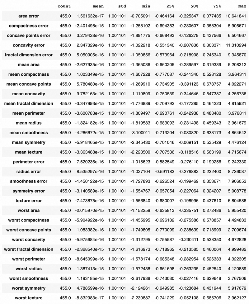
We can see that after using StandardScaler, all the features have zero mean and unit standard deviation.
Let’s get the summary statistics for the training data before standardization as well, and we can see that the mean and standard deviation can be very different in scale. For example, the area error has a mean value of 40 and a standard deviation of 47. On the other hand, the compactness error has a mean of about 0.023 and a standard deviation of 0.019.
# Summary statistics before standardization
X_train.describe().T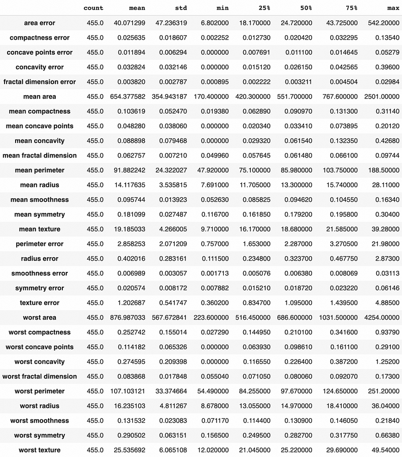
Step 5: Logistic Regression With No Regularization
In step 5, we will create a logistic regression with no regularization as the baseline model.
Logistic regression in sklearn uses Ridge regularization by default. When checking the default hyperparameter values of the LogisticRegression(), we see that penalty='l2', meaning that L2 regularization is used.
# Check default values
LogisticRegression()LogisticRegression(C=1.0, class_weight=None, dual=False, fit_intercept=True,
intercept_scaling=1, l1_ratio=None, max_iter=100,
multi_class='auto', n_jobs=None, penalty='l2',
random_state=None, solver='lbfgs', tol=0.0001, verbose=0,
warm_start=False)We need to change the penalty from l2 to 'none' to get the model with no regularization. After running the baseline logistic regression model, we also predicted the testing dataset using .predict and calculated the predicted probabilities using .predict_proba.
# Run model
logistic = LogisticRegression(penalty='none', random_state=0).fit(X_train_transformed, y_train)
# Make prediction
logistic_prediction = logistic.predict(X_test_transformed)# Get predicted probability
logistic_pred_Prob = logistic.predict_proba(X_test_transformed)[:,1]After getting the predicted value and predicted probability, we are ready to check the model performance!
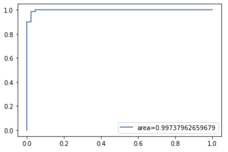
First, let’s check the ROC curve. We got the area under curve value of 0.9818.
# Get the false positive rate and true positive rate
fpr,tpr, _=roc_curve(y_test,logistic_pred_Prob)
# Get auc value
auc=roc_auc_score(y_test,logistic_pred_Prob)# Plot the chart
plt.plot(fpr,tpr,label="area="+str(auc))
plt.legend(loc=4)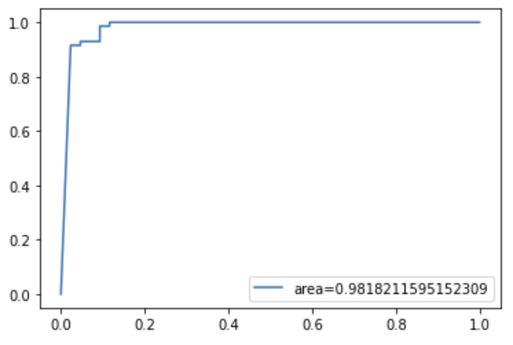
The log loss value for the model is 2.02.
# Caclulate log loss
log_loss(y_test,logistic_pred_Prob)2.0150517046435854The confusion matrix shows 1 false positive and 6 false negatives.
# Confusion matrix
plot_confusion_matrix(logistic, X_test_transformed, y_test)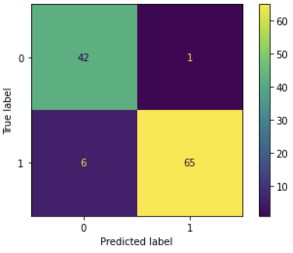
A total of 7 incorrect predictions correspond to an accuracy of 0.939.
We do not want to miss any actual cancer patient for the breast cancer prediction and do not mind having a few false positives, so recall would be the metric to pay most attention to. The recall is the true positive rate. It measures the percentage of actual cancer patients captured by the model. We can see that the logistic regression gave us the recall value of 0.915, meaning that 91.5% of the actual cancer patients are captured.
# Performance report
print(classification_report(y_test, logistic_prediction, digits=3))
precision recall f1-score support 0 0.875 0.977 0.923 43
1 0.985 0.915 0.949 71 accuracy 0.939 114
macro avg 0.930 0.946 0.936 114
weighted avg 0.943 0.939 0.939 114Next, let’s check the coefficients of the model. Based on their absolute values, I ranked the model coefficients from high to low, and we can see the top variables have coefficients in a few hundred.
# Model coefficients
LogisticCoeff = pd.concat([pd.DataFrame(X_test_transformed.columns),
                           pd.DataFrame(np.transpose(logistic.coef_))], axis = 1)
LogisticCoeff.columns=['Variable','Coefficient']
LogisticCoeff['Coefficient_Abs']=LogisticCoeff['Coefficient'].apply(abs)
LogisticCoeff.sort_values(by='Coefficient_Abs', ascending=False)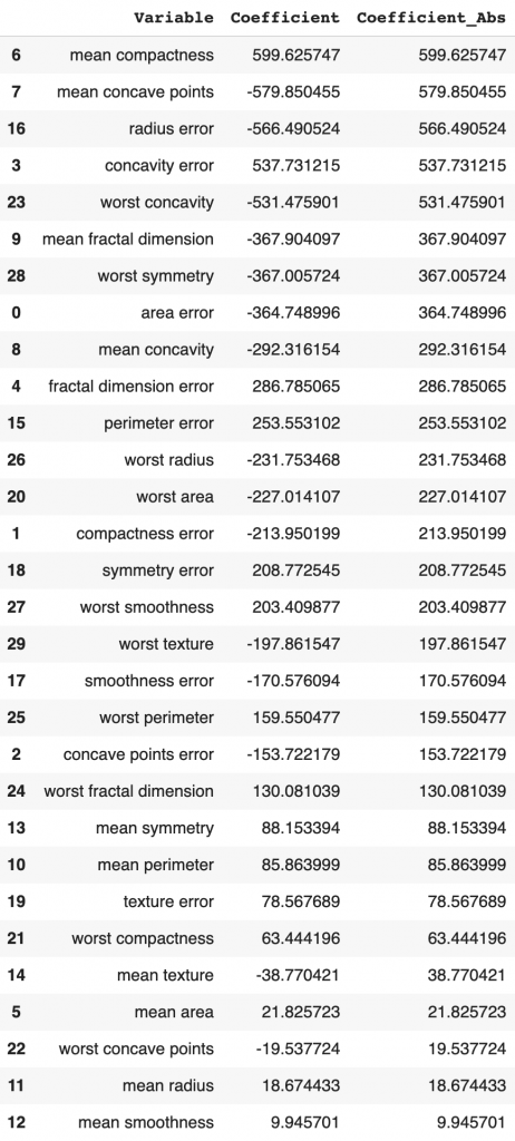
Step 6: LASSO
In step 6, LASSO model is used to run the same analysis.
penalty='l1' means LASSO regularization is applied.
solver is an algorithm to use in the optimization problem. There are different types of solvers. For small datasets, ‘liblinear’ is a good choice, whereas ‘sag’ and ‘saga’ are faster for large datasets.
# Run model
lasso = LogisticRegression(penalty='l1', solver='liblinear',
                           random_state=0).fit(X_train_transformed, y_train)
# Make prediction
lasso_prediction = lasso.predict(X_test_transformed)# Get predicted probability
lasso_pred_Prob = lasso.predict_proba(X_test_transformed)[:,1]The ROC/AUC value is 0.9967 for LASSO, higher than the logistic regression value of 0.9818.
# Get the false positive rate and true positive rate
fpr,tpr, _= roc_curve(y_test,lasso_pred_Prob)
# Get auc value
auc = roc_auc_score(y_test,lasso_pred_Prob)# Plot the chart
plt.plot(fpr,tpr,label="area="+str(auc))
plt.legend(loc=4)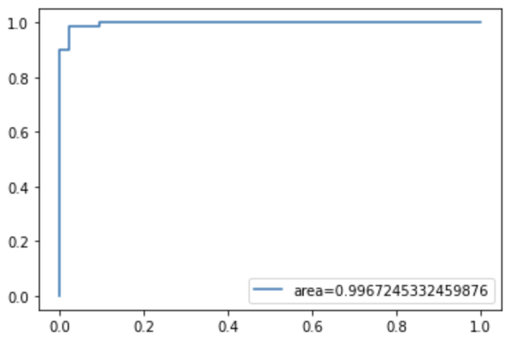
The log loss decreased from baseline logistic regression’s 2.015 to 0.0685. That’s a significant improvement!
# Calculate log loss
log_loss(y_test,lasso_pred_Prob)0.06846705785516008The confusion matrix shows the same false positive count of 1, but the false negative count decreased from 6 to 2.
# Confusion matrix
plot_confusion_matrix(lasso, X_test_transformed, y_test)
Because of the decrease in false-negative count, the accuracy increased from 0.939 to 0.974. And the recall value increased from 0.915 to 0.972.
# Performance report
print(classification_report(y_test, lasso_prediction, digits=3))
precision recall f1-score support 0 0.955 0.977 0.966 43
1 0.986 0.972 0.979 71 accuracy 0.974 114
macro avg 0.970 0.974 0.972 114
weighted avg 0.974 0.974 0.974 114LASSO’s coefficients decreased a lot compared to the logistic regression coefficients. As a result, about half of the features have a coefficient of zero.
So LASSO gives us a simpler model with better performance.
# Model coefficients
lassoCoeff = pd.concat([pd.DataFrame(X_test_transformed.columns),
                       pd.DataFrame(np.transpose(lasso.coef_))], axis = 1)
lassoCoeff.columns=['Variable','Coefficient']
lassoCoeff['Coefficient_Abs']=lassoCoeff['Coefficient'].apply(abs)
lassoCoeff.sort_values(by='Coefficient_Abs', ascending=False)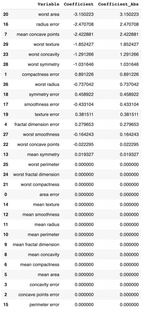
Step 7: Ridge
In step 7, we will run Ridge regression by changing the penalty to l2.
# Run model
ridge = LogisticRegression(penalty='l2', random_state=0).fit(X_train_transformed, y_train)
# Make prediction
ridge_prediction = ridge.predict(X_test_transformed)# Get predicted probability
ridge_pred_Prob = ridge.predict_proba(X_test_transformed)[:,1]# Get the false positive rate and true positive rate
fpr,tpr, _= roc_curve(y_test,ridge_pred_Prob)# Get auc value
auc = roc_auc_score(y_test,ridge_pred_Prob)# Plot the chart
plt.plot(fpr,tpr,label="area="+str(auc))
plt.legend(loc=4)The ROC/AUC value is 0.9974, which is slightly higher than 0.9967 for LASSO.
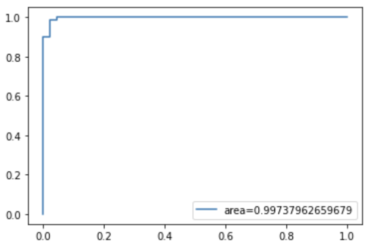
The log loss decreased from LASSO regression’s 0.0685 to 0.0601. That’s an improvement too.
# Calculate log loss
log_loss(y_test,ridge_pred_Prob)0.06014109569918717The confusion matrix shows the same false-positive count of 2 and the false-negative count of 1.
Although the total number of incorrect predictions is 3, the same as LASSO regression, Ridge regression has better performance because the false-negative decreased by 1.
# Confusion matrix
plot_confusion_matrix(ridge, X_test_transformed, y_test)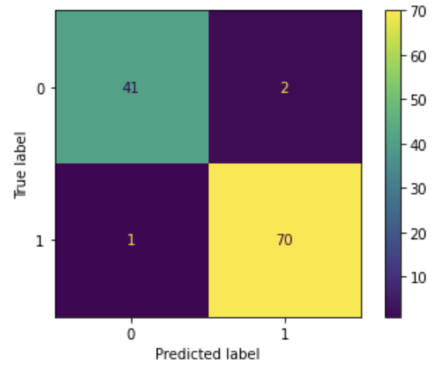
Because the number of incorrect predictions is the same between LASSO and Ridge, the accuracy is the same at 0.974. Because the false-negative count decreased from 2 to 1, the recall value increased from 0.972 to 0.986.
# Performance matrix
print(classification_report(y_test, ridge_prediction, digits=3))
precision recall f1-score support 0 0.976 0.953 0.965 43
1 0.972 0.986 0.979 71 accuracy 0.974 114
macro avg 0.974 0.970 0.972 114
weighted avg 0.974 0.974 0.974 114Ridge’s coefficients decreased slightly compared to the LASSO regression coefficients. Some of the features have a coefficient close to zero, but none of them equals zero.
# Model coefficients
ridgeCoeff = pd.concat([pd.DataFrame(X_test_transformed.columns),
                       pd.DataFrame(np.transpose(ridge.coef_))], axis = 1)
ridgeCoeff.columns=['Variable','Coefficient']
ridgeCoeff['Coefficient_Abs']=ridgeCoeff['Coefficient'].apply(abs)
ridgeCoeff.sort_values(by='Coefficient_Abs', ascending=False)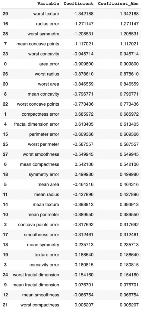
Based on the performance comparison, we can see that Ridge has slightly better performance than LASSO, but LASSO has a simpler model than Ridge.
Step 8: Elastic Net
In step 8, we will run elastic net regression by changing the penalty to 'elasticnet'. l1_ratio=0.5 means that the elastic net uses 50% LASSO and 50% Ridge.
# Run model
elasticNet = LogisticRegression(penalty='elasticnet', solver='saga', l1_ratio=0.5, random_state=0).fit(X_train_transformed, y_train)
# Make prediction
elasticNet_prediction = elasticNet.predict(X_test_transformed)# Get predicted probability
elasticNet_pred_Prob = elasticNet.predict_proba(X_test_transformed)[:,1]# Get the false positive rate and true positive rate
fpr,tpr, _ = roc_curve(y_test,elasticNet_pred_Prob)# Get auc value
auc = roc_auc_score(y_test,elasticNet_pred_Prob)# Plot the chart
plt.plot(fpr,tpr,label="area="+str(auc))
plt.legend(loc=4)The ROC/AUC value for the elastic net is 0.9974, which is about the same as the Ridge regression.
The log loss decreased from Ridge regression’s 0.0601 to 0.0597. That’s a slight improvement.
# Calculate log loss
log_loss(y_test,elasticNet_pred_Prob)0.05970787798591165The confusion matrix shows the same false-negative count of 1, and the false positive count decreased from 2 to 1.
# Confusion matrix
plot_confusion_matrix(elasticNet, X_test_transformed, y_test)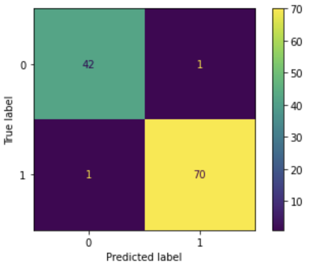
Because the number of incorrect predictions decreased compared to LASSO and Ridge, the accuracy increased from 0.974 to 0.982. The recall value is the same at 0.986.
# Performance report
print(classification_report(y_test, elasticNet_prediction, digits=3))
precision recall f1-score support 0 0.977 0.977 0.977 43
1 0.986 0.986 0.986 71 accuracy 0.982 114
macro avg 0.981 0.981 0.981 114
weighted avg 0.982 0.982 0.982 114Ridge’s coefficients were set to zeros for some features, but the number of features with 0 coefficient is smaller than LASSO.
# Model coefficients
elasticNetCoeff = pd.concat([pd.DataFrame(X_test_transformed.columns),
                             pd.DataFrame(np.transpose(elasticNet.coef_))], axis = 1)
elasticNetCoeff.columns=['Variable','Coefficient']
elasticNetCoeff['Coefficient_Abs']=elasticNetCoeff['Coefficient'].apply(abs)
elasticNetCoeff.sort_values(by='Coefficient_Abs', ascending=False)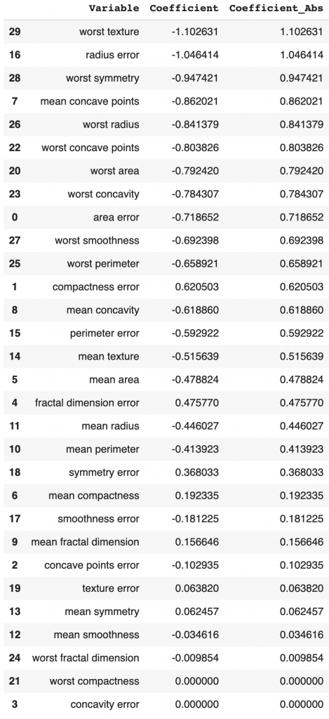
Summary
In this tutorial, we covered
- What’s the difference between LASSO (L1), Ridge (L2), and Elastic Net?
- How to run LASSO for the classification model?
- How to run Ridge for the classification model?
- How to run Elastic Net for the classification model?
- How to compare the performance of LASSO, Ridge, and Elastic Net?
We can see that regularization improved the model performance significantly than not using regularization.
Elastic net has the best performance among the three regularization algorithms, followed by Ridge and LASSO regression. However, this may not be true for all the datasets. Therefore, I suggest trying all three algorithms for your project, doing hyperparameter tuning, and choosing the algorithm that works best for your dataset.
More tutorials are available on GrabNGoInfo YouTube Channel and GrabNGoInfo.com.
Recommended Tutorials
- GrabNGoInfo Machine Learning Tutorials Inventory
- One-Class SVM For Anomaly Detection
- 3 Ways for Multiple Time Series Forecasting Using Prophet in Python
- Four Oversampling And Under-Sampling Methods For Imbalanced Classification Using Python
- Multivariate Time Series Forecasting with Seasonality and Holiday Effect Using Prophet in Python
- How to detect outliers | Data Science Interview Questions and Answers
- Time Series Anomaly Detection Using Prophet in Python
- How to Use R with Google Colab Notebook


