

Credit Card Fraud Detection: A Hands-On Project
Engage in a Machine Learning Project: Credit Card Fraud Detection Through Practical Experience.
Discover:
- Understanding the Significance of Credit Card Fraud Detection
- Introduction to the “Credit Card Fraud Detection” Dataset for the Project
- Building Robust Fraud Detection Models
- Evaluating Model Performance
- Interpreting and Analyzing Model Results
💡I write about Machine Learning on Medium || Github || Kaggle || Linkedin. 🔔 Follow “Nhi Yen” for future updates!
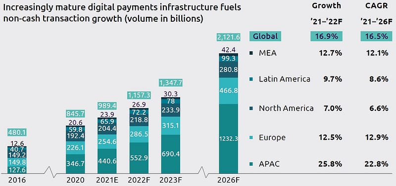
The World Payment Report 2022 highlights the rapid growth of non-cash transactions and the importance of B2B payments value chains and small and medium businesses. Also, it’s expected that in future years there will be a steady growth of non-cash transactions as below
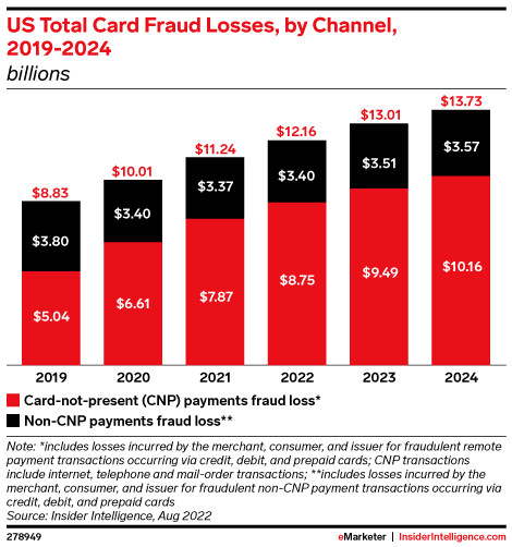
Although it may seem promising, fraudulent transactions have also increased. Despite the implementation of EMV smart chips, a considerable amount of money is still being lost due to credit card fraud.
How can we minimize the risk? Although there are various techniques to decrease losses and prevent fraud, I will guide you through my approach and share my discoveries.
I. About the Dataset
The “Credit Card Fraud Detection” dataset on Kaggle is a highly imbalanced dataset that contains transactions made by credit cards in September 2013 by European cardholders. The dataset includes a total of 284,807 transactions, out of which only 492 are fraudulent, making the dataset highly imbalanced. The dataset includes 28 features, which are numerical values obtained by PCA transformation to maintain the confidentiality of sensitive information. The aim of this dataset is to build a model that can accurately detect fraudulent transactions in real-time to prevent fraudulent activity and reduce the losses incurred by the cardholders and banks. This dataset has been widely used in machine learning research to evaluate different classification algorithms and techniques for dealing with imbalanced datasets.
II. Exploratory Data Analysis
With the data now available, let’s have some checks on the Time, Amount, and Class columns.
1. Time
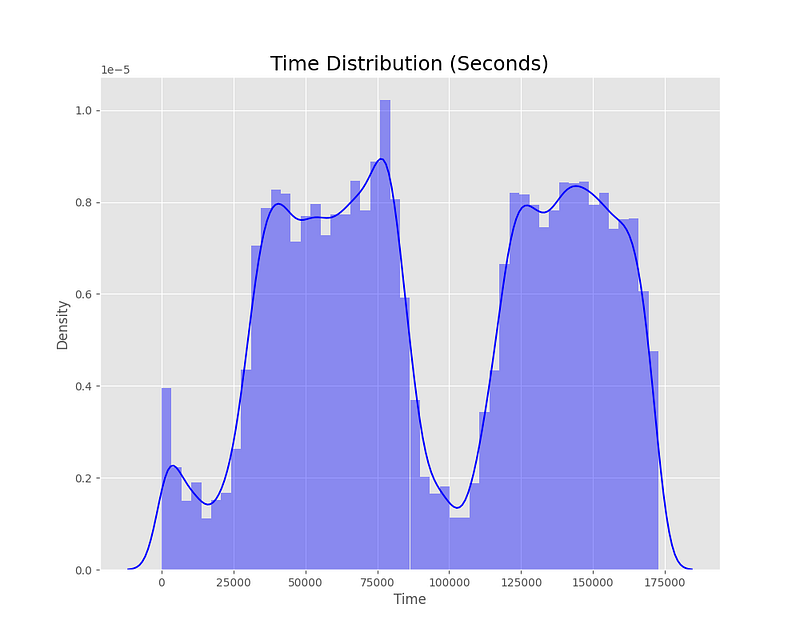
From the plot, we can observe that the Time feature has a bimodal distribution with two peaks, indicating that there are two periods during the day when credit card transactions are more frequent. The first peak occurs at around 50,000 seconds (approximately 14 hours), while the second peak occurs at around 120,000 seconds (approximately 33 hours). This suggests that there may be a pattern in the timing of credit card transactions that could be useful for fraud detection.
2. Amount
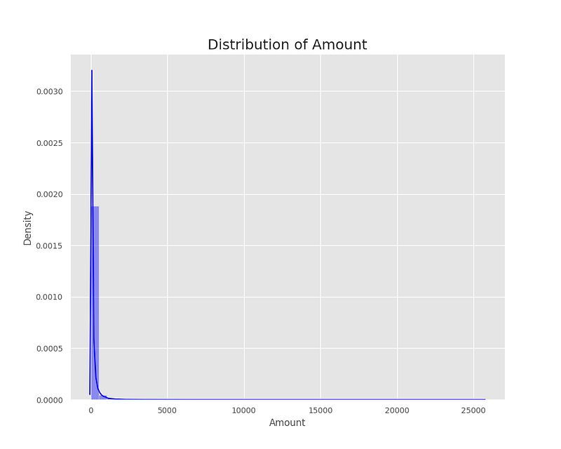
From the plot, we can observe that the distribution of the Amount feature is highly skewed to the right, with a long tail to the right. This indicates that the majority of the transactions have low amounts, while a few transactions have extremely high amounts. As a result, this suggests that the dataset contains some outliers in terms of transaction amounts. Therefore, when building a model for fraud detection, it may be necessary to handle outliers in the Amount feature, for instance, by using a log transformation or robust statistical methods.
3. Class (Fraud | Non-Fraud)
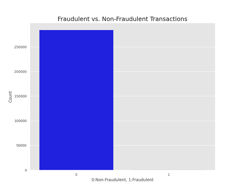
From the plot, we can observe that the dataset is highly imbalanced, with a vast majority of transactions being non-fraudulent (class 0) and a relatively small number of transactions being fraudulent (class 1). This indicates that the dataset has a class imbalance problem, which may affect the performance of a model trained on this dataset. It may be necessary to use techniques such as oversampling, undersampling, or class weighting to handle the class imbalance problem when building a model for fraud detection.
III. Data Processing
To ensure that there wasn’t any significant collinearity in the data, the heatmap was used.
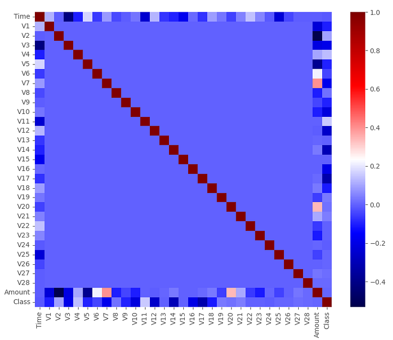
From the heatmap, it can be observed that there are no strong positive or negative correlations between any pairs of variables in the dataset. The strongest correlations are found:
- Time and V3, with a correlation coefficient of -0.42
- Amount and V2, with a correlation coefficient of -0.53
- Amount and V4, with a correlation coefficient of 0.4.
Although these correlations are relatively high, the risk of multicollinearity is not expected to be significant. Overall, the heatmap suggests that there are no highly correlated variables that need to be removed before building a machine learning model.
IV. Modeling
The “Credit Card Fraud Detection” dataset has credit card transactions labeled as fraudulent or not. The dataset is imbalanced, so it needs a model that can accurately detect fraudulent transactions without wrongly flagging non-fraudulent transactions.
To help with classification problems, StandardScaler standardizes data by giving it a mean of 0 and a standard deviation of 1, which results in a normal distribution. This technique works well when dealing with a wide range of amounts and time. To scale the data, the training set is used to initialize the fit, and the train, validation, and test sets are then scaled before running them into the models.
The dataset was divided into 60% for training, 20% for validation, and 20% for testing. To balance the imbalanced dataset, Random Undersampling was used to match the number of fraudulent transactions. Logistic Regression and Random Forest models were used, and good results were produced.
The commonly used models for the “Credit Card Fraud Detection” dataset are Logistic Regression, Naive Bayes, Random Forest, and Dummy Classifier.
- Logistic Regression is widely used for fraud detection because of its interpretability and ability to handle large datasets.
- Naive Bayes is commonly used for fraud detection because it can handle datasets with a large number of features and can provide fast predictions.
- Random Forest is commonly used for fraud detection because it can handle complex datasets and is less prone to overfitting.
- The Dummy Classifier is a simple algorithm used as a benchmark to compare the performance of other models.
P/S: Tony Yiu’s blogs on Logistic Regression and Random Forest were helpful resources in understanding how each one works.
V. Model Evaluation
This section will discuss the following metrics: Accuracy, Recall, Precision, and F1 Score.
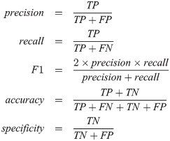
- Accuracy is the fraction of correct predictions the model makes. However, it can be misleading for unbalanced datasets.
- Recall tells us what percentage of fraudulent transactions the model correctly identified. In the best model, the recall is 89.9%, which is a good starting point.
- Precision tells us what percentage of predicted fraudulent transactions were actually fraudulent. In the best model, 97.8% of all fraudulent transactions were captured, which is a good metric.
- F1 Score combines Recall and Precision into one metric as a weighted average of the two, taking false positives and false negatives into consideration. It is much more effective than accuracy for imbalanced classes.
The final results of the trained models are very promising. They have high true positive rates and low false positive rates, which is good for our dataset. Next, we’ll discuss the ROC curve, Confusion Matrix, and how the models compare.
1. ROC Scores
The ROC measures classification performance at different thresholds. A higher AUC score (Area Under the Curve) means the model is better at predicting fraud/non-fraud.
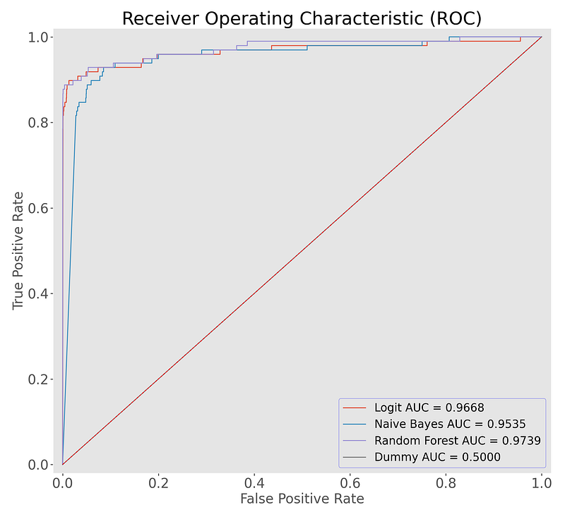
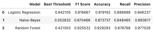
The graph shows AUC scores for Logistic Regression and Random Forest. High scores are good. The points on the curve represent thresholds. Moving right captures more True Positives but also more False Positives. The ideal thresholds are 0.842 for Logistic Regression and 0.421 for Random Forest. At these thresholds, we capture the optimal amount of fraudulent transactions while keeping False Positives low. The Confusion Matrix can visualize the effects of each model.
2. Confusion Matrix — Logistic Regression
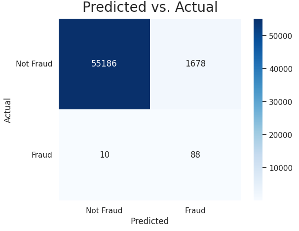
The model captured 88 out of 98 fraudulent transactions and marked 1,678 normal transactions as fraudulent using a threshold of 0.842 in the out-of-sample test set. This is similar to situations when the bank sends a confirmation text after the card is used in another state without prior notice.
3. Confusion Matrix — Random Forest
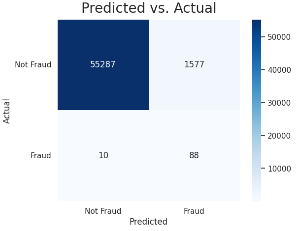
At a threshold of 0.421, the Random Forest model performs similarly to the Logistic Regression model. It correctly identifies 88 out of 98 fraudulent transactions, but it also flags a descrease of normal transactions as fraudulent compared to the Logistic Regression model. Overall, both models have good performance.
Conclusion
Detecting fraudulent credit card transactions is crucial in today’s society. Companies use various methods to capture these instances, and it’s fascinating to see how they deal with this. Finding anomalies is enjoyable, so going through this project was a lot of fun. I hope the findings were explained well, and thanks for reading!
References
- Kaggle Project — HERE
- Github Repo — HERE
- Kaggle Dataset — HERE
- READ MORE — Reproducible Machine Learning for Credit Card Fraud detection — Practical handbook
❗Found the article helpful? Get UNLIMITED access to every story on Medium with just $1/week— HERE
#CreditCardFraudDetection #DataScience #MachineLearning #FraudPrevention #DataAnalysis


