Creating training patches for Deep Learning Image Segmentation of Satellite (Sentinel 2) Imagery using the Google Earth Engine (GEE)

Figure — Example of patch creation for image segmentation of water bodies.

Update

For information about the course Introduction to Python for Scientists (available on YouTube) and other articles like this, please visit my website cordmaur.carrd.co.

Introduction

In some previous stories (here, here and here) we’ve used PyTorch and Fast.ai library to segment clouds in satellite images, using as reference a public dataset (Kaggle’s 38-Cloud: Cloud Segmentation in Satellite Images). However, there are cases when we need to prepare our own dataset from the beginning, and that can be time-consuming without the proper tools.

As it is not my objective here to explain GEE in depth, I will cover just the basics needed to accomplish our final goal, that is to obtain training patches ready to be consumed by any deep learning framework. The workflow I will present here, was done for Sentinel-2 images, but can be easily modified for any other imagery available in the Google Earth Engine platform.

These are the steps:

Select an image from a GEE image collection
Perform a supervised image classification within GEE
Export patches as TensorFlow records (TFRecords). Don’t worry if you don’t use TF (I don’t use it either), because we will convert it to NumPy afterwards.
Open patches in python, and parse them as as NumPy arrays

Selecting an Image in Google Earth Engine

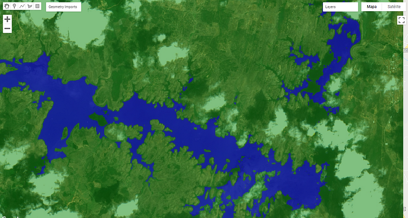
The first thing we need is a free account to the GEE platform, that can be easily obtained in https://signup.earthengine.google.com/. After that, we will go to the code editor (https://code.earthengine.google.com/), and create a new empty script (NEW red button on the left). Within the empty script, copy and paste the following code and hit Run. That would zoom you directly to the Orós reservoir in the northeast of Brazil (Figure 1).

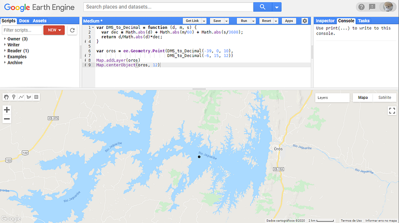
Figure 1 — GEE code editor with a point created in the middle of the Orós reservoir, in Brazil.

To work on a different area, you can adjust the coordinates. A better way (that we will need in the next step, is to create a Point Geometry directly through the interface (Insert Marker button) and center the map on the newly created geometry.

The next step is to select an specific image for our region of interest. To do this we will open an image collection with ee.ImageCollection (S2_SR stands for Sentinel-2, Surface Reflectance — Level 2A products) and filter the images containing the point of interest and that lay within a specific period. We will consider a one-month period and display all the images to inspect them visually (Figure-2). The images will be available in the Layers tool. For this specific search, considering that my objective is to identify water surfaces, the last image (indexed as 3) will be the one used for the next step.

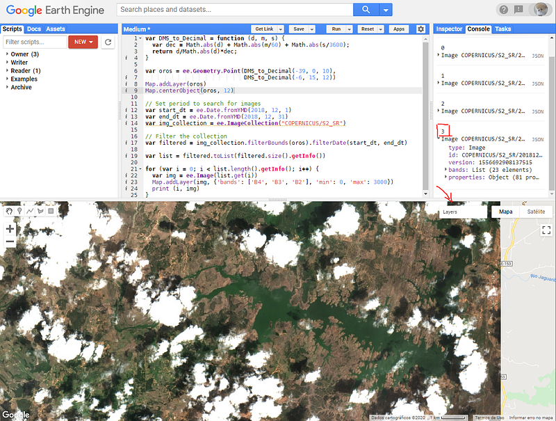
Figure 2 — Selected Sentinel-2 image from Orós reservoir.

Image Classification in GEE

Once we’ve decided the image to work with, we can comment the for-loop that displays the images and stick to the one we are really interested in:

var img = ee.Image(list.get(3))

We will now perform a supervised classification to identify the pixels belonging to the classes we are interested in segmentation. Considering that the focus is water identification, before going into the classification itself, we will create some additional indices that will help the classifier in this task. The indices are the Normalized Difference Water Index (NDWI) and the Modified Normalized Difference Water Index (MNDWI). These indices are created using the normalizedDifference method of GEE and added to our image using addBands, as follows:

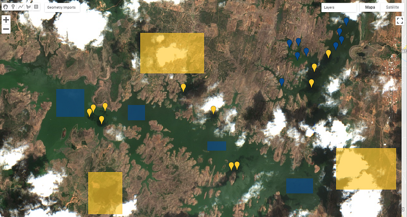
In order to perform a supervised classification in GEE, we need to sample pixels belonging to the classes. Each class should be entered into different layer and the samples can be in form of polygons, rectangles or single markers. In Figure-3 we can see the geometries I created to collect samples for water (blue) and for no-water (yellow). Note that I’ve selected many different targets to be classified as no-water (i.e. clouds, land, shadows, etc.) and also some points in the shadows over water, as I don’t want them to be classified as water.

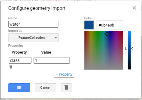
Figure 3 — Sampling regions for the supervised classification (water = blue, not water = yellow).

One additional step that must be done is to create, for each geometry’s layer one property to specify the class for that layer (Figure-4). In this case I created water=1 and no-water=1. This can be done by clicking in Edit Layer button, under Geometry Imports, selecting Import as|FeatureCollection and them adding the desired property.

Figure 4 — Creation of property to hold the class.

Once this is finished, we can run a classifier (ex. Random Forests, Support Vector Machines, etc.) using the samples from these regions as training pixels for each class. The geometry layers will be merged into a collection and we will use the Random Forests classifier. Bellow is the code to merge the regions and run the classifier.

After running the classifier, we can display the layer and set its transparency to 50% to see the final results (Figure 5).

Figure 5 — Classification results in water (blue) and not water (green).

Export image patches

With the image classification ready, we can export the image as patches (equally sized tiles) to fit into a deep learning architecture. If you are like me and find the GEE documentation a bit confusing, here is a step-by-step guide on how to export and then read them as NumPy arrays.

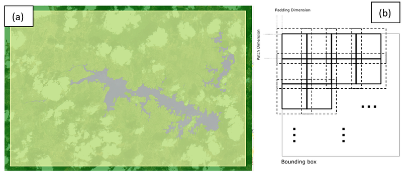
The first thing we will need is a bounding box of the region to be exported. You can export the whole image, but for experimenting, just the reservoir area will be selected. For that, we create a rectangle into a new layer called export_area, over the reservoir (Figure 6a). The patches will be created automatically and exported as a collection of images. Normally there is no overlapping between patches, but one may specify a kernel size (in pixels) that will be used to overlap the patches. This can be useful as a data-augmentation approach, to increase the number of training patches created from a single region.

July, 2020 update: The use of kernel size when exporting overlapping patches from GEE can be tricky if not set up properly and raise an error. The kernel size must be added to the resulting patch size during parsing, as explained in the topic “Opening the patches in Python/NumPy”. I wrote a deeper explanation in the following stackoverflow link: https://stackoverflow.com/questions/62673073/exporting-tfrecords-training-patches-with-google-earth-engine-kernelsize-issues/62939479#62939479

Figure 6b shows the relation between patch dimension and padding dimension, from the GEE documentation.

Figure 6 — Region geometry to be exported (a) and how the tiles are exported (b).

Before exporting the patches we will add the final classification as a new band to the image. We will export the bands used for the classification (bands variable) plus the final classes band.

Also, a variable called export_options will be created to specify the patch dimensions and other parameters. Finally, the patches will be exported to my user’s account Google Drive in TFRecord format. As we are exporting the Orós reservoir, we selected fileNamePrefix as Orós_1 and scale to 10 meters.

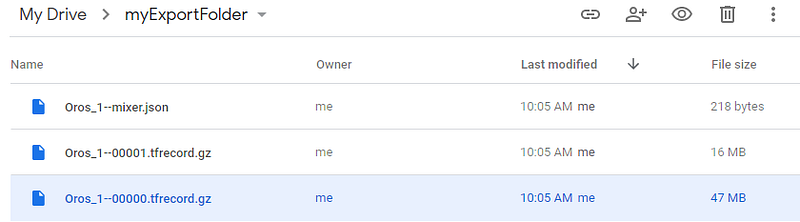
After running this script, the tasks tab (on the right pane) will blink yellow, indicating that the task hasn’t started yet. Go there and hit Run to start exporting the patches to the drive. The export module will also compress the results (if compressed is marked as true) and split it into multiple files according to maxFileSize variable. This can take several minutes depending on the size of the exporting area and when it is finished, the files should appear in the myExportFolder into the Google Drive (Figure 7).

Figure 7 — Exported patches in TFRecord format and compressed into multiple files.

Opening the patches in Python/NumPy

Now that we have the patches exported, we need to convert it (called parse) to be able to use it as NumPy arrays. Considering that the files are saved in the Google Drive, the easiest way to access it using Python is through the Google Colab Platform (https://colab.research.google.com/). If that’s the first time you use it, login with your google account (top right button) and then create a new Notebook (under the files menu).

The first thing we will do is connect the Notebook to the Google Drive and check if our newly created patches are there. There should be a file called *mixer.json that stores the basic properties of the patches like Projection, Patch Dimensions, Patches per Row and others. We will read it just to get the patch dimensions, but this is not mandatory, as we already know the sizes we have specified.

The TFRecordDataset stores the patches with all the bands in serialized structure so, to retrieve the information in a meaningful way, it is necessary to inform how to read each band, for each patch. To do this, we will create a dictionary of the bands we want to extract, and for each band we specify how the TF should read (parse) this band. As we know all the patches share the same shape (100x100) we create a FixedLenFeature for each band. Then, we create a function to parse a single patch using this dictionary and call it through the map method of the dataset (to apply it to all patches).

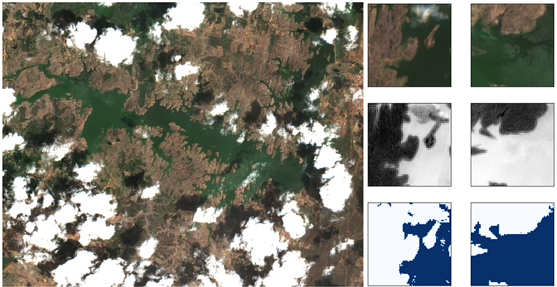
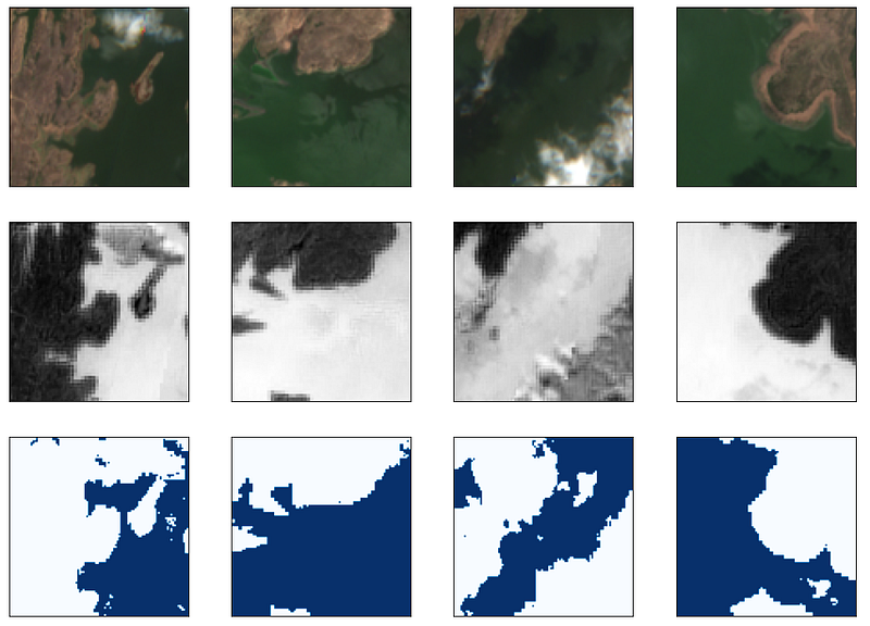
The result of the mapping is MapDataset with the patches and the bands we have exported. To loop through the patches we can use the as_numpy_iterator method. In the last cell of the notebook, I loop through some of them and show an example of the exported patches and it’s corresponding masks (Figure 8). All the code is available in the notebook bellow.

Figure 8 — Patches samples (top) and corresponding MNDWI (middle) and water masks (bottom), where blue is water and white is not water.

As you can see at the end, we can access all the patches and corresponding bands as NumPy arrays and process them normally in any Deep Learning framework. In the next stories I will cover Image Segmentation in Multi-spectral satellite images. Hope you have enjoyed. Should you have any doubt, comments, or a better way to do any of these tasks, share with us in the comments.

See you in the next Story.