Creating an ARIMA Model for Time Series Forecasting

Introducing and implementing the ARIMA model in the AirPassengers dataset

Time-series forecasting consists of making predictions in order to drive future strategic decision-making in a wide range of applications. Based on some of the terms introduced in this previous article such as trend and seasonality, this article focuses on the implementation of autoregressive-, integrated-, moving average-based models for time-series forecasting. Specifically, the structure unfolds as follows:

1. Introduction to the AR, I, MA terms
2. Finding the order of the models
3. Implementation of the ARIMA model
4. Take-home messages

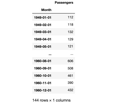
For this article, I have used the Open Database “Air Passengers”, which provides monthly totals of US airline passengers from 1949 to 1960. This dataset includes the rights, without limitation, to sublicense the work and use it for commercial use. The code can be found in the following GitHub repository.

1. Introduction to the AR, I, MA terms

1.1. Autoregression (AR)

The term AR stands for autoregression, which indicates that the model uses the dependent relationship between current data and its past values. The number of preceding inputs used to predict the next value is called order and is usually referred to as p.

In other words, the current value of the series can be explained as a linear combination of the past p values:

where 𝜖𝑡 is a white noise process (mean of 0, constant variance, and uncorrelated errors) and 𝑎𝑖 are the estimated values.

Depending on the value of p, there are the following scenarios:

1. AR(0): If the p parameter is set to zero, there are no autoregressive terms, so this time series is just white noise.
2. AR(1): With the p parameter set to 1, we are taking into account the previous timestamp adjusted by a multiplier, and then adding white noise.
3. AR(p): Increasing the p parameter means adding more timestamps adjusted by their own multipliers.

1.2. Integrated (I)

The I term stands for integrated and makes stationary time series out of your non-stationary one.

Q: Should my time series be stationary to use ARIMA model? [1]

A: If you want to use ARMA(p, q) straightforward, then your time series better be stationary. In practice, there is always some degree of uncertainty about “stationarity”, since you are only observing the realisations, and do not know the real stochastic process random variables. This uncertainty means you just approximately see it’s stationary and try to apply ARMA model, or brute force the d-number, though this will give you subpar performance.

1.3. Moving average (MA)

The Moving Average model uses the dependency between an observation and a residual error from a moving average applied to lagged observation. In other words, MA is modeling the forecast value as a linear combination of the past error terms:

where 𝜖𝑡 is a white noise process (mean of 0, constant variance, and uncorrelated errors), b𝑖 are the estimated values and rt is defined as

where 𝑦̂𝑡 is the prediction value and 𝑦𝑡 is the true value.

2. Finding the order of the models

2.1. Importing the data

Firstly, let’s import the libraries. Note that the version of statsmodels is 0.13.2 (print(statsmodels.__version__)).

For the rest of the article, let’s consider the Air Passengers dataset, which provides monthly totals of US airline passengers from 1949 to 1960.

2.2. Assessing the stationarity of the time-series

A stationary time-series is defined as a time-series whose properties do not depend on the time at which the series is observed. In a more mathematical sense, a time-series is stationary when the covariance is independent of time and it has a constant mean and variance over time. But, why stationarity is important? It is important since many of the model assumptions consider that the time-series is stationary.

The first way of visualizing the trend and seasonality is by representing the rolling mean and rolling average.

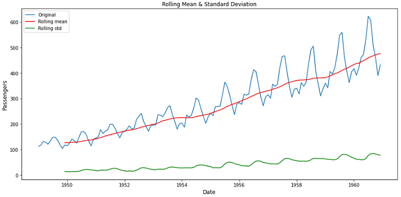
As observed in the figure, there is an increasing trend over time. Also, there is a yearly seasonality component.

Also, the Augmented Dickey-Fuller Test is used to determine if the time-series data is stationary. Similar to the t-test, we set a significance level and draw conclusions based on the resulting p-value.

• Null Hypothesis: The data is not stationary.
• Alternative Hypothesis: The data is stationary.

For the data to be stationary (ie. reject the null hypothesis), the p-value for the ADF test has to be below 0.05.

Results of Dickey-Fuller Test:
Test Statistic                   0.815369
p-value                          0.991880
Lags Used                       13.000000
Number of Observations Used    130.000000
Critical Value (1%)             -3.481682
Critical Value (5%)             -2.884042
Critical Value (10%)            -2.578770
dtype: float64

Results indicate that the p-value is 0.992, meaning that it is very likely that the data is not stationary.

The following function decomposes the time-series into the trend, seasonal and residual components, so it can be also used to study the stationarity of the time-series.

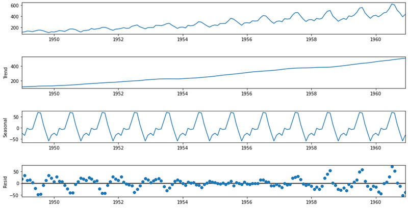
In the figure, we can also observe the yearly seasonality and the increasing trend over time.

But, what happens if the time-series is stationary? In that case, it is necessary to convert the data into a stationary time-series.

In general, it is a good practice to follow the next steps when doing time-series forecasting:

• Step 1 — Check Stationarity: If a time series has a trend or seasonality component, it must be made stationary.
• Step 2 — Determine the d value: If the time series is not stationary, it needs to be stationarized through differencing.
• Step 3 — Select AR and MA terms: Use the ACF and PACF to decide whether to include an AR term, MA term, (or) ARMA.
• Step 4 — Build the model

Steps 3 and 4 are covered in Sections 2.4–2.7, whereas Step 5 is covered in Section 3.

2.3. Selecting training and test sets

Before continuing, let’s create a training and test set to avoid having a bias in the forecasting prediction.

2.4. Finding the value of the d (Integrated) parameter

If the data is not stationary, it is necessary to find the integrated parameter that makes the time-series into stationary.

Since there is not a method that can tell us the optimal d value, let’s plot the first-order and second-order differencing:

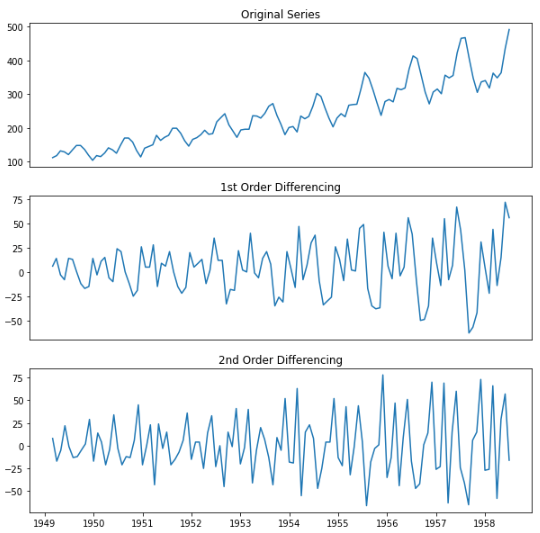
After implementing differencing on the time-series, both the trend and seasonality have been reduced.

It is also possible to assess the optimal d value using the autocorrelation plots. When there is a trend in the data, the autocorrelations for small lags tend to be large and positive, slowly decreasing over time as the lags increase. When there is a seasonality component within the time-series, the autocorrelations will be larger for the seasonal lags (at multiples of the seasonal frequency) than for other lags.

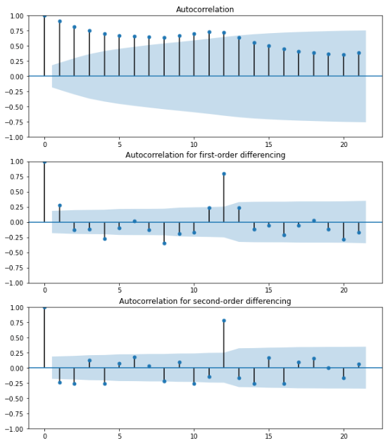
Here we can see that in second-order differencing the immediate lag has gone on the negative side, representing that in the second-order the series has become over the difference. Hence, we will select the first-order differencing.

2.5. Finding the value of the p (Autoregressive) parameter

In the previous section, we have identified the optimal value of d. Now, in this section, let’s find the optimal number of autoregressive terms by inspecting the PACF plot.

The partial autocorrelation function plot can be used to draw a correlation between the time series and its lag. Significant correlation in a stationary time series can be represented by adding autoregression terms. Using the PACF plot we can take as the AR terms the lags that are significant.

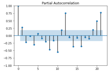
As there are many lags that are significant, we can select a high number of autoregressive terms.

2.6. Finding the value of the q (Moving average) parameter

To find out the value of q, we can use the ACF plot, expressed as:

where T is the length of the time series, and k is the lag applied to the time series.

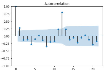
Here we see that the second lag is already out of the significance limit.

To have a deeper understanding of the definitions of PACF and ACF, I strongly recommend reading the following article.

2.7. Using the auto_arima to find the parameters

Lastly, just mentioned that there is a function that seeks to identify the most optimal parameters for an ARIMA model, settling on a single-fitted ARIMA model.

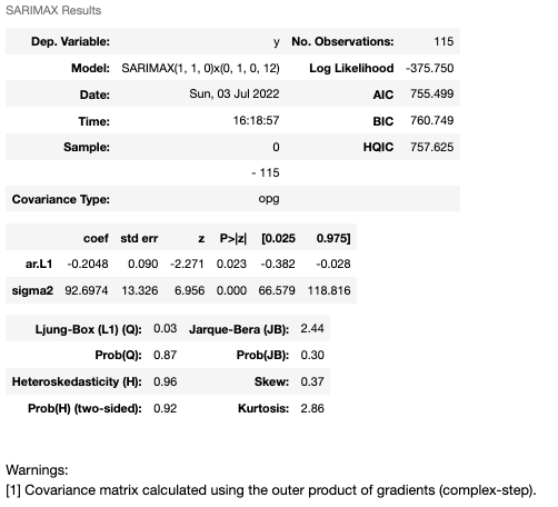
However, this output is related to the SARIMAX model which is not covered in this article. Hence, we will omit the results obtained and focus on the analysis implemented above.

3. Implementation of the ARIMA model

The most suitable model will depend on the particular characteristics of the data such as trend and seasonality. In this article, we focus on the implementation of the ARIMA model.

Using the parameters (p=12, d=1, q=1) derived from the previous analysis, let’s check the output:

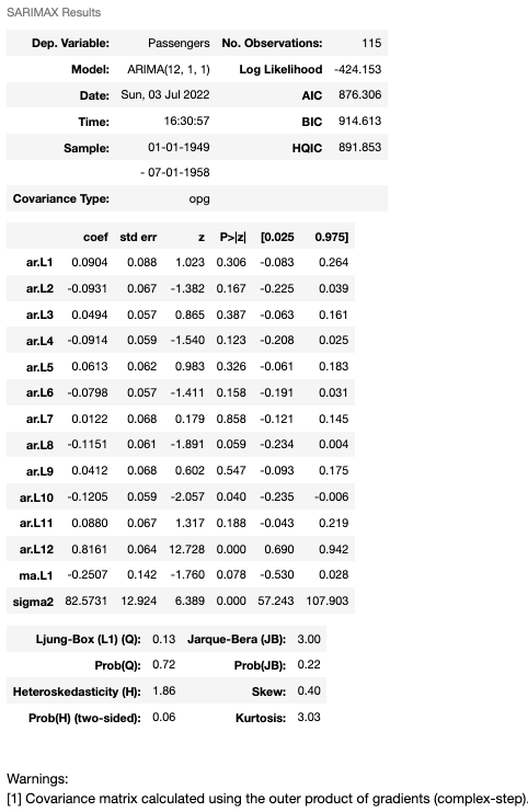
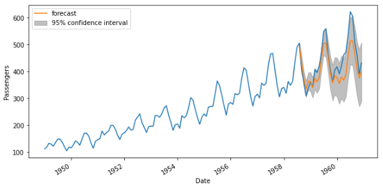
Here is the output, where the orange line indicates the forecasting and the gray shadow is the prediction intervals, which are used to provide a range where the forecast is likely to be with a specific degree of confidence [3].

4. Take-home messages

In this article, we have discussed the process of finding the values of parameters in the ARIMA modeling. Before concluding the article, here are the main tips to remember:

• The autoregressive model (AR) uses past forecasts to predict future values.
• The I term stands for integrated and makes stationary time series out of your non-stationary one.
• The moving average (MA) model doesn’t use past forecasts to predict future values whereas it uses the errors from the past forecasts.
• Use PACF to determine the terms used in the AR model and the ACF to determine the terms used in the MA model
• We can go as far back as we want for selecting the AR(p) term, but as we get further back it is more likely that we should use additional parameters such as the moving average (MA(q)).

If you enjoyed this post, please consider subscribing. You’ll get access to all of my content + every other article on Medium from awesome creators!

References

[1] StackExchange, Should my time series be stationary to use ARIMA model?

[2] Otexts, Stationarity and differencing

[3] Medium, Time-series forecasting prediction intervals

Important references

• Nist, Model Identification
• Medium, A Step-by-Step Guide to Calculating Autocorrelation and Partial Autocorrelation
• Medium, Find the order of ARIMA models
• Medium, Time Series Forecasting: Prediction Intervals
• Otexts, ARIMA

Other:

• Medium, ARIMA for dummies
• Kaggle, Store Sales Forecasting ARIMA and AUTOARIMA
• Machine Learning Mastery, How to Create an ARIMA Model for Time Series Forecasting in Python