ARIMA for dummies

While at work, developing reinforcement learning model I’ve came across an Auto regressive model that is used to update policy in RL agent. This activated very deep and un-visited part of my brain which is “already learned” part. I’ve remembered that I’ve written a blog on using ARIMA which is combination of AutoRegressive model with Moving Average model. I thought it would be good idea to recap my understanding and also bring out my blog into the light. So here it goes.

Before going in to ARIMA we must recap on what “Time Series” is.

Time Series

Data points that are observed at specified times usually at equal intervals are referred to as time series data. Time series is very important in real life since most data are measured in time consecutive manner. Ex: Stock prices being recorded every second.

Time series analysis are used to predict the future. For example using past 12 months sales data to predict next n month sales therefore we could act accordingly.

Four components that explains time series data:

1. Trend : Upward, downward, or stationary. If your company sales increase every year it is showing an upward trend.
2. Seaonality: Repeating pattern in certain period. Ex: difference between summer and winter. Also includes special holidays
3. Irregularity: External factors that affect time series data such as Covid, natural disasters.
4. Cyclic: repeating up and down time series data.

ARIMA

Auto Regressive Integrated Moving Average a.k.a Box-Jenkins method.

• It is class of models that forecasts using own past values: lag values and lagged forecast errors.
• AR model uses lag values to forecast
• MA model uses lagged forecast errors to forecast
• Two models Integrated becomes ARIMA (“I” stands for Integrated)
• Consists of three parameters: p, q, d

ARIMA a naive model, it assumes time series data we are working with satisfies following conditions:

1. “non-seasonal” meaning different seasons do not affect its values. When there exists seasonality we use SARIMA short for Seasonal ARIMA model
2. No Irregularity. Ex: No irregular events like Covid that affect our data

Now we know what ARIMA model is and what it expects lets talk about what parameters it has in more detail

Parameters

p — order of AR term

• Number of lags of Y to be used as predictors. In other words, If you are trying to predict June’s sale how many previous(lag) month’s data are you going to use?

q — order of MA term

• Number of lagged forecast errors -> how many past forecast errors will you use?

d — Minimum differncing period

• Minimum number of differencing needed to make time series data stationary.
• Already stationary data would have d = 0.

While reading about explanation of each parameters term Stationary was not clear on my mind therefore after some research I’ve gained knowledge to answer my question:

What does stationary actually mean?

Time series data considered stationary if it contains:

1. constant mean
2. constant variance
3. Covariance that is independent of time

In most cases time series data increase as time progresses therefore if you take consecutive segments it will not have constant mean. Below graph is Nvidia stock prices which is an example of non-stationary data. Segment into n periods and take means, they won’t be the same.

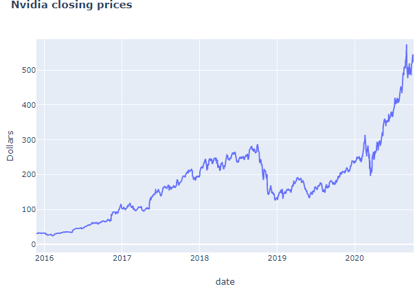
It is important to check whether our data is stationary because time series data need to be stationary before it can be modelled to forecast the future. Often times it is non-stationary therefore we difference it, subtract previous value from current value.

Since it is important to have stationary time series data, we need a way to test it. Common methods of testing whether time series data is stationary are:

• Augmented Dickey Fuller(ADF) Test
• Phillips-Perron(PP) Test
• Kwiatkowski-Phillips-Schmidt-Shin(KPSS) Test
• Graphing rolling statistics such as mean, standard deviation

Model building in python

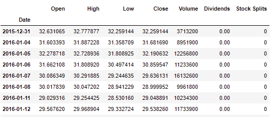
We will be using python 3.8 to build ARIMA model and predict Nvidia’s closing stock prices.

First thing we must do, check if data is stationary. From the line graph we’ve seen earlier of Nvidia’s closing stock prices it is quite clear that it is not stationary however to make sure it is always a good practice to test it.

We will test it using Augmented Dickey Fuller Test. To test if data is stationary, we use hypothesis testing where our null hypothesis would be “time series data is non-stationary”. We will reject null hypothesis when p-value is less than 0.05(p-value) which makes us take alternative hypothesis “time series data is stationary”.

Notice that our null hypothesis is rejected because p-value ≥ 0.05. So now we know our data is not stationary however it doesn’t end here because we can make it stationary by using technique called “differencing”.

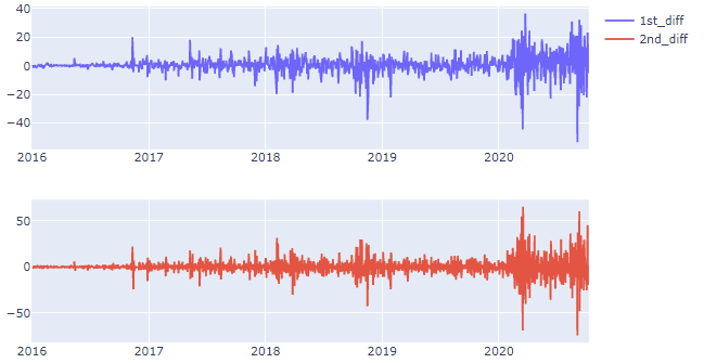
Just by using 1st order differencing we can see that our data became stationary.

Below is auto-correlation plot of 1st order differencing. You can see that even with one lag it lead to negative auto-correlation right away which indicates over-differencing. When auto-correlation decrease too fast it may indicate over-difference and if auto-correlation decrease too slow(stays positive for more than 10 lags) it indicates under-differencing.

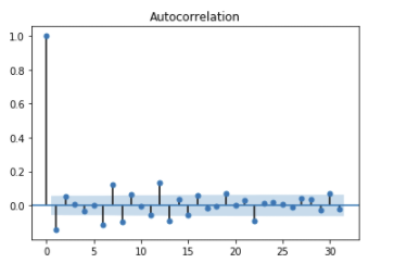
Also when time series is slightly under differenced, differencing once more lead to slight over differencing and vice versa. In such case instead of differencing add AR terms when slightly under-differenced and add MA terms when slightly over-differenced.

Forecasting with ARIMA

Finally time to use ARIMA model to make prediction. There is manual way to select q,d,p however since blog is getting too long I will explain it more deeper in later blogs and will show you easy way to select parameters.

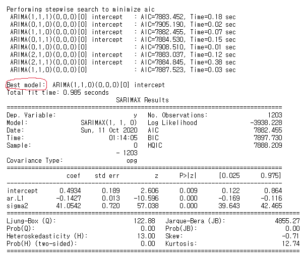
Above code tries all combination of p,d,q and output best model which is model with lowest AIC. Now create best ARIMA model and make predictions. Note that since it is time series data order matters therefore must split train and test data sequentially.

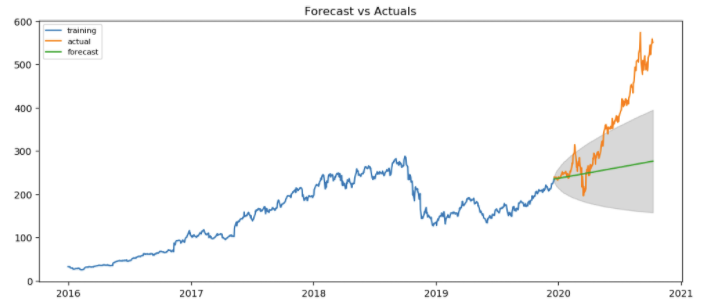
Above graph proves that our prediction doesn’t do a good job. This is because ARIMA model does not account for irregularity and since Nvidia price sky rocketed due to events like CES and rise of self-driving vehicles our ARIMA model did a poor job.

Up to October 2018 there seems to be no irregularities. When we truncate our data to include data until October 2018 we get following forecast.

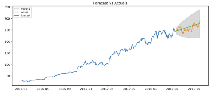
We can see that our ARIMA model actually does a great job when there are no irregularity(one of assumptions).

In conclusion, ARIMA works well when we are working with data with no irregularity and no seasonality. There are more robust versions of ARIMA such as SARIMAX(Seasonal ARIMA model with eXogenous variable) which works w/o assumptions that are made by ARIMA. I usually work in bottom-up fashion therefore I always try to keep things simple therefore start with building simplest base model which in our case is ARIMA, than move up to SARIMA and SARIMAX.

References

• https://www.machinelearningplus.com/time-series/arima-model-time-series-forecasting-python/#:~:text=ARIMA%2C%20short%20for%20'Auto%20Regressive,used%20to%20forecast%20future%20values
• https://www.youtube.com/watch?v=e8Yw4alG16Q&t=2047s
• https://machinelearningmastery.com/time-series-data-stationary-python/