Courage to Learn ML: A Detailed Exploration of Gradient Descent and Popular Optimizers

Are You Truly Mastering Gradient Descent? Use This Post as Your Ultimate Checkpoint

We will use an RPG game as an analogy today. Created By ChatGPT

Welcome back to a new chapter of ‘Courage to Learn ML. For those new to this series, this series aims to make these complex topics accessible and engaging, much like a casual conversation between a mentor and a learner, inspired by the writing style of “The Courage to Be Disliked,” with a specific focus on machine learning.

In our previous discussions, our mentor and learner discussed about some common loss functions and the three fundamental principles of designing loss functions. Today, they’ll explore another key concept: gradient descent.

As always, here’s a list of the topics we’ll be exploring today:

What exactly is a gradient, and why is the technique called ‘gradient descent’?
Why doesn’t vanilla gradient descent perform well in Deep Neural Networks (DNNs), and what are the improvements?
A review of various optimizers and their relationships (Newton’s method, Adagrad, Momentum, RMSprop, and Adam)
Practical insights on selecting the right optimizer based on my personal experience

So, we’ve set up the loss function to measure how different our predictions are from actual results. To close this gap, we adjust the model’s parameters. Why do most algorithms use gradient descent for their learning and updating process?

To address this question, let’s imagine developing a unique update theory, assuming we’re unfamiliar with gradient descent. We start by using a loss function to quantify the discrepancy, which encompasses both the signal (the divergence of the current model from the underlying pattern) and noise (such as data irregularities). The subsequent step involves conveying this data and utilizing it to adjust various parameters. The challenge then becomes determining the extent of modification needed for each parameter. A basic approach might involve calculating the contribution of each parameter and updating it proportionally. For instance, in a linear model like W*x + b = y, if the prediction is 50 for x = 1 but the actual value is 100, the gap is 50. We could then compute the contribution of w and b, adjusting them to align the prediction with the actual value of 100.

However, two significant issues arise:

Calculating the Contribution: With many potential combinations of w and b that could yield 100 when x = 1, how do we decide which combination is better?
Computational Demand in Complex Models: Updating a Deep Neural Network (DNN) with millions of parameters could be computationally demanding. How can we efficiently manage this?

These difficulties highlight the complexity of the problem. It’s nearly impossible to accurately determine each parameter’s contribution to the final prediction, especially in non-linear and intricate models. Therefore, to update model parameters effectively based on the loss, we need a method that can precisely dictate the adjustments for each parameter without being computationally costly.

Thus, rather than focusing on how to allocate loss across each parameter, we could consider it as a strategy to traverse the loss surface. The objective is to locate a set of parameters that guide us to the global minimum — the closest approximation achievable by the model. This adjustment process is akin to playing an RPG game, where the player seeks the lowest point in a map. This is the foundational idea behind gradient descent.

We have a set of basic movements to guide our hero towards finding the treasure, which is located at the lowest point in the map. Created by ChatGPT

So what is exactly gradient descent? Why it call gradient descent?

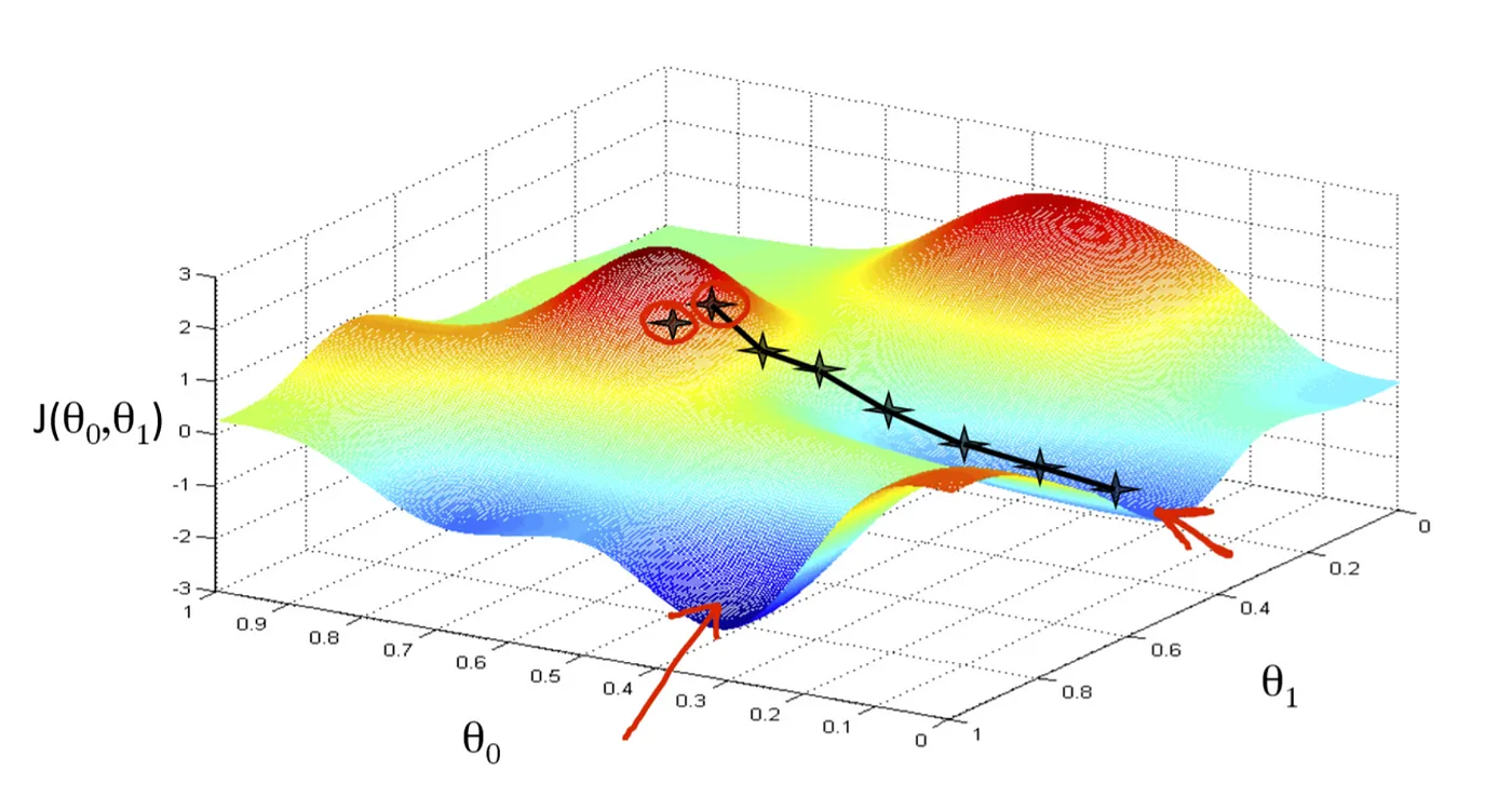
Let’s break it down. The loss surface, central to optimization, is shaped by the loss function and model parameters, varying with different parameter combinations. Imagine a 3D loss surface plot: the vertical axis represents the loss function value, and the other two axes are the parameters. At the global minimum, we find the parameter set with the lowest loss, our ultimate target to minimize the gap between actual results and our predictions.

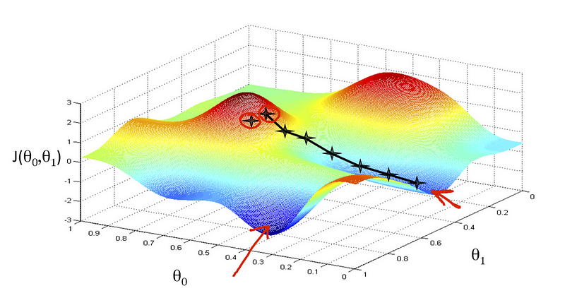
Source: https://miro.readmedium.com/v2/resize:fit:1400/format:webp/1*DDjCOEPSHLsU7tff7LmYUQ.png

But how do we navigate towards this global minimum? That’s where the gradient comes in. It guides us in the direction to move. You might wonder, why calculate the gradient? Ideally, we’d see the entire loss surface and head straight for the minimum. But in reality, especially with complex models and numerous parameters, we can’t visualize the entire landscape — it’s more complex than a simple valley. We can only see what’s immediately around us, like being in a foggy landscape in an RPG game. So, we use the gradient, which points towards the steepest ascent, and then head in the opposite direction, towards the steepest descent. By following the gradient, we gradually descend to the global minimum on the loss surface. This journey is what we call gradient descent.

How exactly does gradient descent decide the adjustments needed for each parameter, and why is it more effective than our initially proposed simple method?

Our objective is to minimize the loss function with a particular set of parameters, achievable only by adjusting these parameters. We indirectly influence the loss function through these changes.

Let’s revisit our RPG analogy. The hero, with only basic movements (left/right, forward/backward) and limited visibility, aims to find the lowest point on an uncharted map to unearth a legendary weapon. We know the gradient indicates the direction to move, but it’s more than just a pointer. It also decomposes into fundamental movements.

The gradient, a vector of partial derivatives with respect to each parameter, signifies how much and in which basic direction (left, right, forward, backward) to move. It’s like a magical guide not only pointing to the hill’s left side will lead us to the legendary weapon but also instructing specific turns and steps to take.

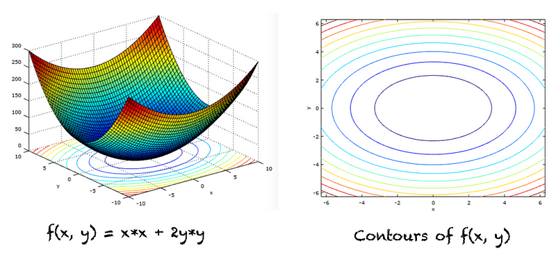
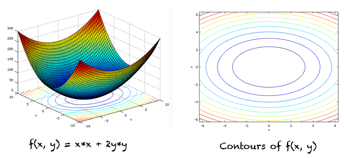
However, it’s crucial to understand what the gradient actually is. Often tutorials suggest imagining you’re on a hill and looking around to choose the steepest direction to descend. But this can be misleading. The gradient isn’t a direction on the loss surface itself but a projection of that direction onto the parameter dimensions (in the graph, the x,y coordinates), guiding us in the loss function’s minimal direction. This distinction is crucial — the gradient isn’t on the loss surface but a directional guide within the parameter space.

The vector v represents the gradient and can be expressed in the coordinate form determined by our parameters x and y. Source: https://eli.thegreenplace.net/images/2016/plot-3d-parabola.png

That’s why most visualizations use parameter contours, not the loss function to illustrate gradient descent processes. The movement is about adjusting parameters, with changes on the loss function being a consequence.

Source: https://machinelearningmastery.com/wp-content/uploads/2021/07/gradientDescent1.png

Gradient is formed by partial derivatives. A partial derivative, on the other hand, helps us understand how a function changes in relation to a specific parameter, holding others constant. This is how gradients quantify each parameter’s influence on the loss function’s directional change.

Gradient descent naturally and efficiently resolves the parameter tuning dilemma we initially faced. It’s especially adept at locating global minima in convex problems and local minima in nonconvex scenarios. Modern implementations benefit from parallelization and acceleration via GPUs or TPUs. Variations like mini-batch gradient descent and Adam optimize its efficiency across different contexts. In summary, gradient descent is stable, capable of handling large datasets and numerous parameters, making it a superior choice for our learning purposes.

In the gradient descent formula 𝜃 = 𝜃 — 𝜂⋅∇𝜃𝐽(𝜃), we use the learning rate (𝜂) multiplied by the gradient (∇𝜃𝐽(𝜃)) to update each parameter. Why is the learning rate necessary? Wouldn’t adjusting the parameter directly with the gradient be faster?

At first glance, using only the gradient to reach the global minimum seems straightforward. However, this overlooks the gradient’s nature. The gradient, a vector of partial derivatives of the loss function with respect to parameters, indicates the direction of steepest ascent and its steepness. Essentially, it guides us in the most promising direction given our limited perspective, but it’s just that — a direction. We must decide how to act on this information.

The learning rate, or step size, is crucial here. It controls the pace of our learning process. Imagine the character at the top of a mountain in our video game example. The game indicates that moving left and downhill is the quickest way to the treasure (representing the global minimum). It also informs you about the hill’s steepness: a steepness of 5 to the left and 10 forward. Now, you decide how far to move your hero. If you’re cautious, you might choose a small step, say a learning rate of 0.001. This means your hero moves 0.0015 = 0.005 units to the left and 0.00110 = 0.01 units forward. As a result, your hero moves towards the goal, aligned with the gradient’s direction but at a controlled pace without overshooting.

To sum up, it’s important not to confuse the gradient’s magnitude with the learning pace. The magnitude indicates the steepness of the ascent direction, which can vary depending on the loss surface. The learning rate, on the other hand, is a choice you make, independent of the dataset. It’s a hyperparameter, signifying how cautiously or aggressively we want to proceed in our learning journey.

If the learning rate isn’t dependent on the dataset, how do we determine it? What’s the typical range for a learning rate, and what are the issues with setting it too high or too low?

Since the learning rate is a hyperparameter, we typically choose it through experimentation, like cross-validation, or based on previous experience. The common range for learning rates is between 0.001 and 0.1. This range is based on empirical observations from the data science community, who have found that learning rates within this range tend to converge faster and more effectively. Theoretically, we prefer a learning rate no higher than 0.1 because larger rates can alter our parameters too drastically at each step, leading to risks like overshooting. On the practical side, we avoid rates lower than 0.001 as they can slow down the learning process, making it computationally expensive and time-consuming.

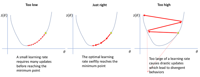
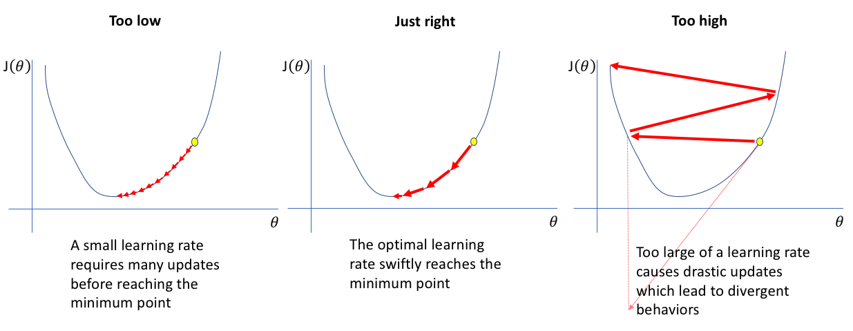
The common range gives us insights into the problems with extreme learning rates. When the rate is too high, the large step size might cause the algorithm to move too fast, leading to overshooting and never reaching the goal. Conversely, a very low rate results in tiny steps, potentially taking an excessive amount of time to reach the global minimum, thus wasting computational resources and time.

Here’s a visual representation to help understand the impact of different learning rates on the learning process:

Source: https://www.jeremyjordan.me/content/images/2018/02/Screen-Shot-2018-02-24-at-11.47.09-AM.png

What are the limitations of vanilla gradient descent, especially when applied to DNN models?

Even though gradient descent works well in theory, it faces significant challenges in practical applications, particularly with DNN models. The key limitations include:

Vanilla gradient descent is computationally intensive. The vanilla gradient descent formula 𝜃 = 𝜃 — 𝜂⋅∇𝜃𝐽(𝜃) requires calculating the average loss 𝐽(𝜃) across the entire dataset. This means comparing all predicted values with their true labels and averaging these differences. For a typical DNN model, which often involves millions of parameters and large datasets, this process becomes computationally intense. This complexity is one of the reasons why practical applications of DNNs weren’t feasible until the advent of models like AlexNet in 2012, despite gradient descent being a much older concept.
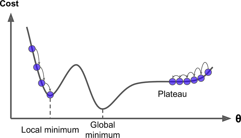
The loss surface in DNNs, usually non-convex, contains multiple local minimums. The simplistic criterion of using gradient descent to find points where 𝐽(𝜃) = 0 is inadequate in such scenarios. In our video game analogy, this is like our hero being unsure of where to move next, as the steepest descent direction becomes indiscernible. Particularly problematic are plateau and saddle points, where 𝐽(𝜃) is zero. The areas that are close to saddle and local minimums can be even harmful, since in those areas 𝐽(𝜃) is very small and close to zero. The small value of 𝐽(𝜃) can significantly slow down the learning process, consuming time and computational resources unnecessarily.

Keep in mind that in the foggy landscape scenario, we have no idea whether we’re on a plateau, at a global minimum, or a local minimum. Source: https://miro.readmedium.com/v2/resize:fit:1400/1*vx235JUNzgv0fGzONlNIYg.png

Why does gradient descent work, and why must the learning rate be small?

Author’s Note: I debated whether to include this section in my post, knowing that mathematical formulas can be intimidating. Yet, while exploring gradient descent, I found myself questioning why the direction of the steepest descent is believed to lead to the global minimum and why tutorials emphasize setting a small learning rate to prevent overshooting. My attempts to rationalize these concepts through RPG game analogies were helpful but not entirely satisfying. It was the straightforward mathematical proof behind gradient descent that finally put my doubts to rest. If you’ve had similar questions, I encourage you to read this section. It might just offer the clarity you need to grasp these concepts fully.

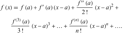
To grasp gradient descent, we need to discuss approximating the loss function using Taylor series. The Taylor series is an incredibly powerful tool for estimating the value of a complex function at a specific point. It’s like trying to describe a complex situation using simpler, individual elements. Instead of using a broad statement like “I had a car accident,” you break it down into specific events: driving the dog to the vet, the dog popping up in the backseat, the phone ringing, and then the crash. The Taylor series does something similar. Instead of trying to describe a complex function f(x) with a single general term, it uses a series of terms to describe the specific value of f(x) at x = a. Taylor series breaks down a function into a sum of polynomial terms based on the function’s derivatives at a specific point (x = a). Each term of the series adds more detail to the approximation.

For an engaging explanation of the Taylor series and how the first and second derivatives contribute to its expansion, check out 3Blue1Brown’s video on Taylor series. It effectively demonstrates why these derivatives are often sufficient for a solid approximation around the point of interest.

Now, returning to our objective of minimizing the loss function, 𝐽(𝜃), we can apply the Taylor series, primarily relying on the first derivative for an effective approximation. In this context, 𝐽(𝜃) is a multivariable function, where 𝜃 is a vector representing a set of parameter variables, and a is the current value of these parameters.

To minimize 𝐽(𝜃), we can only adjust (𝜃 — a) to be really small, meaning our next set of 𝜃 values must be very close to our current position, represented by vector a. This necessity for proximity is why a small learning rate is crucial. If 𝜃 deviates significantly from the current parameter values a, minimizing our loss function becomes challenging. Additionally, since the gradient 𝐽’(a) indicates a direction, we choose (𝜃 — a) to move in the opposite direction. This approach explains why following the direction of the steepest descent (opposite to the gradient) steers us towards the global minimum, where 𝐽(𝜃) = 0.

You particularly mentioned that vanilla gradient descent isn’t ideal for DNNs. Why?

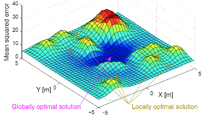
The core issue with applying vanilla gradient descent to DNNs lies in the nature of their loss functions, which are typically non-convex. Gradient descent struggles in these scenarios. Imagine navigating a complex map that isn’t just a simple hill or valley but a terrain filled with unpredictable elevations and depressions. In such a landscape, gradient descent may fail to guide us to the global minimum and might even increase the loss function’s value after parameter updates. This is partly because first-order partial derivatives provide limited information, showing how the loss changes with respect to one parameter while holding others constant. But this doesn’t account for interactions between multiple parameters, which are crucial in complex models.

Source: https://www.researchgate.net/publication/334986617/figure/fig1/AS:789459528335363@1565233227897/Illustration-of-the-non-convex-mean-squared-error-cost-function-of-a-two-dimensional.png

Revisiting the Taylor series concept from our previous discussion, we see that when the objective or loss function becomes highly complex, using only the first derivative doesn’t provide an accurate approximation. Hence, vanilla gradient descent is less effective in navigating complex, non-convex loss functions.

It’s important to note that gradient descent can still reduce the loss in non-convex scenarios. It’s a general method for continuous optimization and can be applied to nonconvex functions, where it will converge to a stationary point. However, this point might not be the global minimum but could be a local minimum or even a saddle point, depending on the function’s convexity.

How can we improve upon vanilla gradient descent to accelerate reaching the global minimum?

Great question! Our previous discussions and the video game analogy reveal several ways to refine gradient descent. Let’s explore these enhancements:

Making the map more player-friendly.

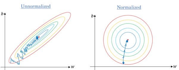
Just like navigating a more accommodating map in a game makes reaching the treasure easier, certain modifications can make the path to the global minimum smoother in gradient descent. This includes using techniques like feature selection, regularization, and feature scaling. Feature selection not only reduces computational costs but also simplifies the loss surface, as the loss surface is influenced by the number of parameters. L1/L2 regularization can help in this process: L1 for feature selection and L2 for smoothing the loss surface. Feature scaling is crucial because features on different scales can cause uneven step sizes, potentially slowing down convergence or preventing it altogether. By scaling features to similar ranges, we ensure more uniform steps, facilitating faster and more consistent convergence.

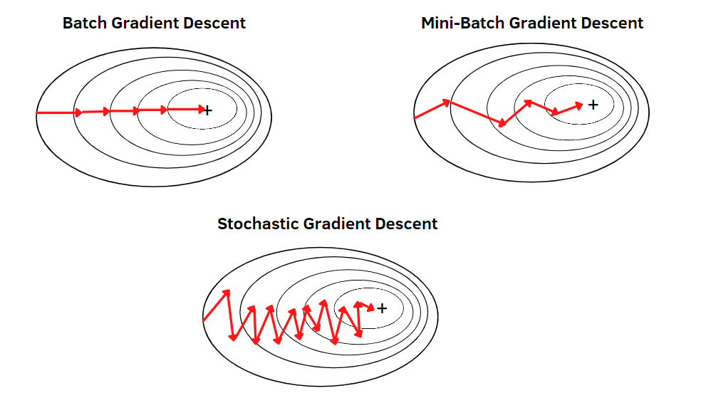
Source: https://qph.cf2.quoracdn.net/main-qimg-591ce5575f71110585d9246bf8c2ca0b-pjlq

Move faster.

There’s a Chinese saying, “天下武功无快不破” (no martial art is indestructible, except for speed). This concept applies to gradient descent as well. In vanilla gradient descent, calculating the loss use the whole training data in each iteration is time-consuming and resource-intensive. However, we can achieve similar results with less data. The idea is that the average loss from a smaller sample is not significantly different from the entire dataset. By employing methods like mini-batch gradient descent (using a subset of data) or Stochastic Gradient Descent (SGD, selecting a random sample each time), we can speed up the process significantly. These approaches enable quicker computations and updates, making them particularly effective in DNNs.

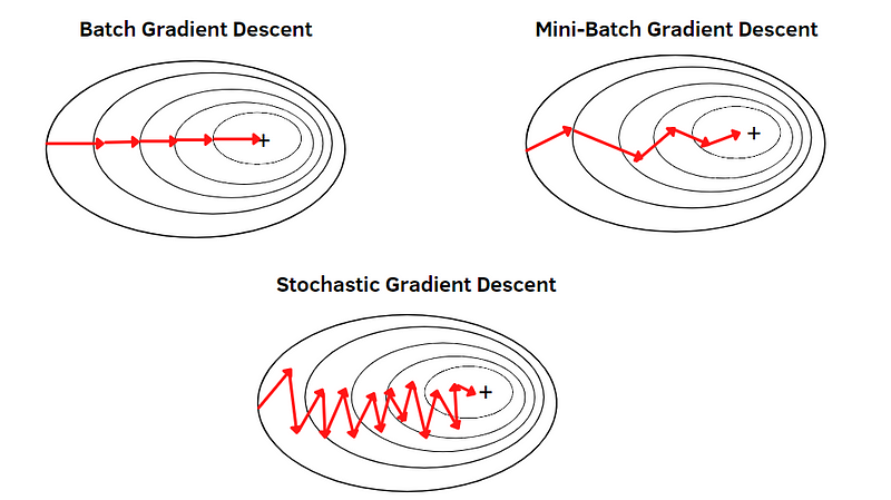
Source: https://editor.analyticsvidhya.com/uploads/58182variations_comparison.png

In the world of machine learning, the term ‘SGD’ (Stochastic Gradient Descent) has evolved to generally refer to any variant of gradient descent that uses a small subset of data for each run. This includes both the original form of SGD and mini-batch gradient descent. Conversely, ‘batch gradient descent’ denotes the approach where the entire training dataset is used for each gradient descent iteration.

Here are some common terms you’ll encounter in discussions about gradient descent:

Batch Size: This is the number of observations (or training data points) used for one iteration of gradient descent.

Iterations per epoch: This indicates how many gradient descent iterations are required to go through the entire dataset once, given the current batch size.

Epoch: An epoch represents one complete pass through the entire training dataset. The number of epochs is a choice made by the modeler and is independent from both the batch size and the number of iterations.

To illustrate, consider a training dataset with 1000 observations. If you opt for a batch size of 10, you’ll need 1000/10 = 100 iterations to cover the entire dataset once. If you set your epoch count to 5, the model will go through the entire dataset 5 times. This means a total of 5 * 100 = 500 gradient descent iterations will be performed.

Move smarter by gathering more information.

Moving smarter in gradient descent involves looking beyond just the steepest descent. In our previous session on the mathematics behind gradient descent, we learned that using the first derivative of f(x) at x = a provides a solid approximation of f(x). However, to enhance this approximation, incorporating additional derivative terms is beneficial. In our video game analogy, this equates to not just finding the steepest descent direction but also moving our camera around to gain a comprehensive understanding of the landscape. This approach is particularly useful for identifying whether we’re at a local/global minimum (like being at the bottom of a valley), or a maximum (at the top of a hill), or a saddle point (surrounded by hills and valleys). However, our limited view means we can’t always distinguish between a local and a global one.

Expanding on this concept, we can apply Newton’s Method. This technique calculates both the first and second derivatives of the objective or loss function. The second derivatives create the Hessian matrix, offering a more detailed view of the loss function’s landscape. With information from both the first and second derivatives, we gain a closer approximation of the loss function. Unlike traditional gradient descent, Newton’s Method doesn’t use a learning rate. However, variations such as Newton’s method with line search do include a learning rate, adding a level of adjustability. While Newton’s Method might seem more efficient than vanilla gradient descent, it’s not commonly used in practice due to its higher computational demands. For more insights into why Newton’s Method is less prevalent in machine learning, you can refer to the discussion here.

Adjust step size while moving around.

This strategy can make our journey more efficient. The simplest approach is to reduce the step size as we approach the global minimum. This is particularly relevant in gradient descent variants like SGD, where the learning rate decreases with each epoch (via learning rate schedules). However, this method uniformly adjusts the learning rate across all parameters, which might not be ideal given the complexity of the loss landscape. In the realm of video games, this is akin to varying the intensity of different movements to navigate more effectively. That’s where methods like Adagrad come in, offering an adaptive gradient approach. It does so by accumulating the history of squared gradients for each parameter and using the square root of this accumulation to adjust the learning rate individually. This method is like fine-tuning our actions in the game based on past experiences, especially when unusual updates occur.

However, while intuitive, Adagrad can slow down due to its aggressive rate decay. Variations of this method seek to balance this aspect.

There are two ways to understand why Adagrad use the sum of squared gradients. Firstly, it allows more cautious learning when the current gradient is significantly larger than historical ones. If we encounter a substantially larger gradient at a given time, adding its squared value to the decay term increases the term significantly, leading to a smaller learning rate and more cautious updates. Secondly, this approach approximates the magnitude of the function’s second derivatives. A larger sum of squared first derivatives suggests a steeper surface, indicating the need for smaller steps.

Choosing better basic movements.

Optimizing our moves in gradient descent involves refining our approach based on the landscape. In vanilla gradient descent, our path often zigzags, similar to uncertain steps in a video game. This can be visualized with the contour of two parameters showing more vertical movements and fewer horizontal ones, even though a horizontal path might be more efficient.

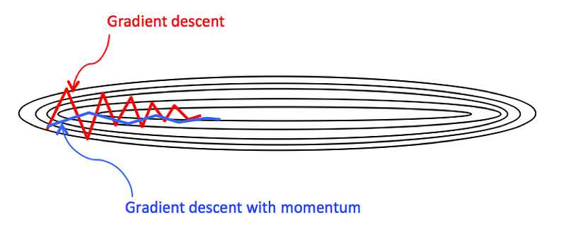
Feature scaling can help, but with the complex surfaces in DNNs, a more directed approach is needed. This is where Momentum Gradient Descent comes into play. It identifies if movements in certain directions are counterproductive. Instead of directly updating parameters with the current gradient, it calculates an exponential moving average of past gradients. This ‘momentum’ helps accelerate progress in consistent directions and dampens movements in unproductive ones.

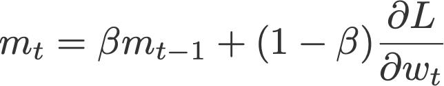
Notice here, unlike Adagrad which uses squared gradients, we accumulate the historical gradients directly. This approach is crucial because it allows for the positive and negative movements to cancel out each other. Think of this as building momentum in a specific direction, accelerating the learning process if we consistently move in a similar direction. Conversely, a small accumulated value suggests little progress in that direction, hinting that it may not be the most promising movement toward the minimum.

To enhance this smoothing effect and capitalize on past movements, we assign more weight to the accumulated gradient history. This is done by setting a higher value for the momentum coefficient, typically denoted as β. A common choice for β is 0.9, which strikes a balance between giving importance to historical movements while still being responsive to new gradient information. This method ensures a smoother journey by favoring directions with consistent progress and dampening oscillations that do not contribute effectively towards reaching the goal.

Combine those strategies!

Merging the principles of Adagrad and Momentum Gradient Descent offers an innovative way to enhance gradient descent. Both these methods rely on historical gradients, but with a key difference in their approach. Momentum Gradient Descent uses the exponential moving average of gradients instead of a simple average. The advantage here is that by adjusting the momentum coefficient β, we can strike a balance between the influence of historical gradient trends and the current gradient.

Inspired by this, we can apply a similar logic to Adagrad, leading to the development of RMSprop (Root Mean Square Propagation). RMSprop is essentially an evolved version of Adagrad, utilizing the exponential moving average of historical gradients rather than a simple average. This modification places more weight on historical gradients, reducing the impact of exceptionally large current gradients. Consequently, it leads to a less aggressive decrease in the learning rate, addressing the issue of slow learning rates that Adagrad often faces.

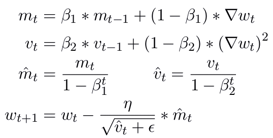
Building further on this idea, why not combine the learning rate adjustment of Adagrad/RMSprop with the gradient adjustment strategy of Momentum? This thought led to the creation of Adam (Adaptive Moment Estimation, I remember it as the baby of Adaptive learning rate and Momentum). Adam essentially combines these two methods by using historical gradients in two ways: one for adjusting the exponential moving average (momentum), and the other for managing the scale of historical gradients (RMSprop). This dual application makes Adam a highly effective and stable optimizer. Adam is a popular choice of optimizer, even though it introduces two additional hyperparameters for fine-tuning.

With various optimizers available, how should one choose the right optimizer in practice?

In practice, choosing the right optimizer depends on the specifics of your data and learning objectives. Here are some of general guidelines from my observations and experience:

SGD for Online Learning: Online learning involves processing a continuous stream of incoming data, which requires frequent updates to the model with new, small data batches. Stochastic Gradient Descent (SGD) is particularly well-suited for this scenario as it efficiently uses small batches for more frequent model updates compared to other optimizers. Additionally, SGD is effective in environments where data is unstable or experiencing minor shifts. Using an appropriate learning rate to avoid overshooting, SGD can quickly adapt the model to subtle changes in data. However, it’s important to note that while SGD is capable of handling non-stationary environments, it may not be as effective in capturing major shifts in data patterns.
Adam and sparse data. When dealing with data that has a high number of zero entries, it’s described as being sparse. The challenge with sparse data lies in the limited information available for certain features. Adam optimizer is particularly effective in this context as it integrates both momentum and adaptive learning rate mechanisms. This combination allows Adam to tailor the learning rate for each parameter individually. Consequently, it provides more frequent updates for features that are underrepresented or have less information due to the data’s sparsity, ensuring a more balanced and effective learning process.
Don’t combine optimizers, but use them together wisely. While it’s possible to use multiple optimizers in the learning process, they shouldn’t be applied simultaneously within a single learning phase, as this can lead to confusion in the model and complicate the learning path. Instead, there are two strategic approaches to effectively utilizing multiple optimizers:
Switching between optimizers at different stages. For instance, when training DNNs, you might begin with Adam for its rapid progress capabilities in the initial epochs. Later, as the training progresses, switching to SGD in the subsequent epochs can offer more precise control over the learning process, aiding the model in converging to a more optimal local minimum.
Using different optimizers to train different parts of a model. In scenarios where new layers are added to an existing, pre-trained model, a nuanced approach can be beneficial. For the pre-trained layers, a stable and less aggressive optimizer is ideal for maintaining the integrity of the already learned features. In contrast, for the newly added layers, an optimizer that’s more aggressive and facilitates faster learning adjustments would be more suitable. This method ensures that each part of the model receives the most appropriate optimization technique based on its specific learning requirements.

Wait, why can’t we use Adam and SGD together? And why is SGD often preferred in later epochs for finer optimization, even though Adam is considered more advanced?

Adam and SGD differ significantly, especially in how they manage the learning rate. While Adam uses an adaptive learning rate, SGD typically employs a fixed rate or a scheduled adjustment. This distinction makes them fundamentally different optimizers.

Adam’s ability to adjust the learning rate doesn’t always make it “more advanced”. In some cases, simiplicity is better. SGD’s simple learning rate and steady approach are more effective, particularly in later epochs. Adam may reduce the learning rate too aggressively, leading to instability, whereas SGD’s consistent rate can more reliably approach a better local minimum and enhance stability.

Furthermore, SGD’s slower convergence can help prevent overfitting. Its fine-grained and controlled adjustments allow for a more precise fit to training data, potentially improving generalization to unseen data. The fixed or scheduled learning rate of SGD also offers researchers better control over the model’s learning process, emphasizing preferences on precision and stability over speed, especially in the final phases of model tuning.

If you’re enjoying this series, remember that your interactions — claps, comments, and follows — do more than just support; they’re the driving force that keeps this series going and inspires my continued sharing.