
Convolutional Neural Network: Step-by-Step Implementation in PyTorch
PyTorch is one of the most popular deep learning frameworks

Convolutional neural networks (CNNs) have played a key role in the history of artificial intelligence (AI). These networks demonstrate substantial performance using these networks in various applications including object classification, object detection, language translation, human re-identification and self-driving vehicles.
CNNs were among the first deep neural networks that provide a sense of vision to a machine. In this article, I will explain how to implement a convolutional neural network for the object classification task using PyTorch which is one of the most popular deep learning frameworks based on Python.
A convolutional neural network is built with four types of layers: Convolutional Layer, Pooling Layer, Rectified Linear Unit (ReLU) layer and Fully-Connected Layer. Let’s see how can we build a convolutional neural network step-by-step using PyTorch.
For this post, I am using the MNIST dataset and I am using the default PyTorch’s datasets package to use the public MNIST dataset. If you would like to use your own dataset for the image classification task, you can read my other post titled “Deep Transfer Learning — Classify your own data set using PyTorch” where I used a custom dataset to implement transfer learning.
I have divided the implementation procedure of a cnn using PyTorch into 7 steps:
Step 1: Importing packages
Step 2: Preparing the dataset
Step 3: Building a CNN
Step 4: Instantiating the model
Step 5: Creating loss function and optimizer
Step 6: Training the network
Step 7: Plotting loss and accuracy curve
Now, I would like to explain each step so that one can understand the implementation easily.
Step 1: Importing packages
We will utilize torchand its subsidiaries torch.nn and torch.nn.functionl. We will also use torchvision for preparing dataset. We will use matplotlib for plotting the loss and accuracy curves.
# Step 1: Import packages

import torch
import torchvision
import torch.nn.functional as F
import torch.nn as nn
import torch.optim as optim
import torchvision.transforms as transforms
import matplotlib.pyplot as plt
Step 2: Preparing dataset
Before feeding the dataset into a convolutional neural network, we need to process the dataset into a format that is suitable for PyTorch. In this post, I used build-in high-quality datasets from the PyTorch libraries. That’s why I do not need to think too much about the pre-processing of the dataset here. I used the MNIST dataset which is included in torchvisionmodule. Before feeding data into a network, we must normalize it. This helps to maintain data within a range and reduces skewness, allowing the network to learn more quickly and efficiently. We also need to pass the dataset through torch.utils.data.DataLoaderto access the data.
# Step 2: Prepare the dataset

transform = transforms.Compose([
                                transforms.Resize(28,28),
                                transforms.ToTensor(),
                                transforms.Normalize([0.1307], [0.3081])


])

train_dataset = torchvision.datasets.MNIST(root='./data/MNIST', train=True, download=True, transform=transform)
val_dataset = torchvision.datasets.MNIST(root='./data/MNIST', train=False, download=True, transform=transform)

train_loader = torch.utils.data.DataLoader(train_dataset, batch_size=32, shuffle=True)
val_loader = torch.utils.data.DataLoader(val_dataset, batch_size=32, shuffle=False)
Step 3: Building a CNN
This step is so exciting because we are going to build our own designed convolutional neural network. We are building the CNN consisting of two convolutional layers. We build a class named Net, where we define the structure of our network. It is noted that the MNIST dataset has 10 classes. That’s why the fully connected layer’s output dimension is 10.
# Step 3: Build a CNN
class Net(nn.Module):
    def __init__(self, num_classes=10):
      super().__init__()
      self.conv1 = nn.Conv2d(in_channels=1, out_channels=20, kernel_size=5, stride=1, padding=0)
      self.conv2 = nn.Conv2d(in_channels=20, out_channels=50, kernel_size=5, stride=1, padding=0)
      self.fc1 = nn.Linear(4*4*50, 500)
      self.dropout1 = nn.Dropout(0.5)
      self.fc2 = nn.Linear(500, num_classes)
    def forward(self, x):
      x = self.conv1(x)
      x = F.relu(x)
      x = F.max_pool2d(x, 2, 2)
      x = self.conv2(x)
      x = F.relu(x)
      x = F.max_pool2d(x, 2, 2)
      x = x.view(-1, 4*4*50)
      x = F.relu(self.fc1(x))
      x = self.dropout1(x)
      x = self.fc2(x)
      return x
If you have a Graphics processing unit (GPU) on your machine, you can enable GPU acceleration for computing in the simplest way using the following code.
# make sure to enable GPU acceleration if you have GPU on your machine
device = 'cuda'
Step 4: Instantiating the model
In this step, we instantiate the convolutional neural network. It is important to transfer the model to the GPU if you would like to use GPU for the acceleration of the computation.
# Step 4: Instantiate the model
model = Net()
model.to(device)
Step 5: Creating a loss function and optimizer
We’ll now construct the loss function and optimizer. We’re employing cross-entropy loss and the Adam optimizer in this case. Cross-entropy loss is a metric for evaluating the performance of a classification model whose output is a probability value between 0 and 1.
On the other hand, adam is a first- and second-order moment estimation stochastic gradient descent algorithm that calculates the gradient’s 1st-order moment (the gradient mean) and 2nd-order moment (element-wise squared gradient) and corrects its bias using exponential moving average.
# Step 5: Create a loss function and optimizer
criterion = nn.CrossEntropyLoss()
optimizer = torch.optim.Adam(model.parameters(), lr = 3e-4)
Step 6: Training the network
In this step, we will pass all the training data to the model. This is called a forward pass. When we will pass the data through the model, we will calculate the loss using cross-entropy loss which we defined earlier step. Based on the loss calculation, the optimizer will update the weights and biases. We will keep track of the training and validation loss and accuracy so that we can plot the loss and accuracy curve in the next step.
#Step 6: Training the Network
# Do a forward pass
# Calculate loss
# Calculate gradients
# Update the weights based on the computed gradients


# keep track of loss and accuracy

training_loss_history = []
training_corrects_history = []
val_loss_history = []
val_corrects_history = []
for e in range(20):

  running_loss = 0.0
  running_corrects = 0.0
  val_running_loss = 0.0
  val_running_corrects = 0.0

  # train the model #

  for inputs, labels in train_loader:
    # Move the training data to the GPU
    inputs = inputs.to(device)
    labels = labels.to(device)

    # forward propagation
    outputs = model(inputs)

    # calculate the loss
    loss = criterion(outputs, labels)

    # clear previous gradient computation
    optimizer.zero_grad()

    # backpropagate to compute gradients
    loss.backward()

    # update model weights
    optimizer.step()

    #predictions
    _, preds = torch.max(outputs, 1)

    #update running loss
    running_loss += loss.item()

    # update runnung accuracy
    running_corrects += torch.sum(preds == labels.data)

  # validate the model

  else:
    with torch.no_grad():
      for val_inputs, val_labels in val_loader:
        # Move the training data to the GPU
        val_inputs = val_inputs.to(device)
        val_labels = val_labels.to(device)

        # forward propagation
        val_outputs = model(val_inputs)

        # calculate the loss
        val_loss = criterion(val_outputs, val_labels)

        # predictions
        _, val_preds = torch.max(val_outputs, 1)

        # update val running loss
        val_running_loss += val_loss.item()

        # update val accuracy
        val_running_corrects += torch.sum(val_preds == val_labels.data)

    # Calculate Training loss
    epoch_loss = running_loss/len(train_loader.dataset)
    training_loss_history.append(epoch_loss)

    # Calculate Training Accuracy
    epoch_acc = running_corrects.float()/ len(train_loader.dataset)
    training_corrects_history.append(epoch_acc)

    # Calculate validation loss
    val_epoch_loss = val_running_loss/len(val_loader.dataset)
    val_loss_history.append(val_epoch_loss)

    # Calculate validation accuracy
    val_epoch_acc = val_running_corrects.float()/ len(val_loader.dataset)
    val_corrects_history.append(val_epoch_acc)

    # Priniting the epoch, loss and accuracy
    print('epoch :', (e+1))
    print('training loss: {:.4f}, Training accuracy {:.4f} '.format(epoch_loss, epoch_acc.item()))
    print('validation loss: {:.4f}, validation accuracy {:.4f} '.format(val_epoch_loss, val_epoch_acc.item()))
Step 7: Plotting loss and accuracy curve
This step is important sometimes. If you draw the loss or accuracy curve for the training and validation data, you will know when the training process would be stopped and you will also be able to know that is there any overfitting that occurs or not.
# plot the training and validation loss
plt.plot(training_loss_history, label='training loss')
plt.plot(val_loss_history, label='validation loss')
plt.suptitle('Training loss vs Test loss', fontsize=16)
plt.xlabel('epoch', fontsize=12)
plt.ylabel('loss', fontsize=12)
plt.legend()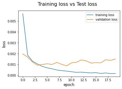
#plot the training and validation accuracy
plt.plot(training_corrects_history, label='training accuracy')
plt.plot(val_corrects_history, label='validation accuracy')
plt.suptitle('Training Accuracy vs validation Accuracy', fontsize=16)
plt.xlabel('epoch', fontsize=12)
plt.ylabel('accuracy', fontsize=12)
plt.legend()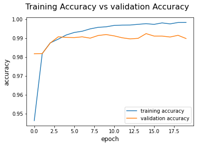
Please find the whole code here.
CNN is one of the fundamental topics of deep learning. This post will help you to understand the implementation procedure of a CNN using the PyTorch deep learning framework.
If you enjoyed my writing please consider sharing it around, following me on Facebook, Twitter, Youtube, or Instagram, or throwing some money into my tip jar on Ko-fi or Paypal. You can also support me by becoming a member on Medium for just $5 a month using my referral link: