
Deep Transfer Learning — Classify Your Own Dataset using PyTorch
Using a pre-trained model on your own data set
In this post, I will discuss deep transfer learning. I will also talk about how to classify images of flowers by using transfer learning from a pre-trained network using PyTorch (one of the most popular deep learning frameworks).
Transfer learning is one of the most important tools of machine learning. Deep neural networks require lots of labeled data in order to get good performance. However, in most cases, we do not have enough data to train a deep network from scratch. In this situation, we are using transfer learning for a particular task.
A pre-trained model is a saved network that was trained earlier on a large data set. Transfer learning for image classification is based on the idea that if a model is trained on a large and general enough data set, it may successfully serve as a generic model of the visual world. You may then use these learned feature maps to train a large model on a large data set without having to start from scratch.
In practice, very few people train a deep neural network from scratch since it is relatively difficult to have a large data set of a sufficient number of samples of each category. Instead, it is a common practice among the machine learning folks to pre-train a deep neural network on a large data set, for example, the ImageNet data set that has 1.2 million images with 1000 classes, and then use the pre-trained model on a small data set for a particular task such as classification images.
The strategy comprises employing an existing neural network that has been trained to perform well on a larger data set as the foundation for a new model that leverages the accuracy of the prior network for a similar task. This approach has gained popularity day by day as a way of improving the performance of a deep neural network trained on a small data set.
Without further ado, let’s implement transfer learning using PyTorch. In this post, I am going to classify flower images. I am using Google Colab to train the network. It is noted that Colab provides a graphics processing unit (GPU) facility for free. Now I will talk about the implementation of deep transfer learning step by step using PyTorch and Colab. If you use Colab, please change the GPU option to accelerate the hardware from the runtime option of Colab.
Now, let’s see how many steps are needed.
Steps:
- Download datasets and unzip
- Import necessary libraries
- Set hyper-parameters
- Set the device
- Prepare the dataset
- Instantiate the model
- Create a loss function and optimizer
- Training the network
- Predict the classes of all the test images
- Class wise test accuracy for all test images and confusion matrix
- Plot the train and validation loss and accuracy curve
- Classify an image from the web using our model
- Visualize the classification results with data
I will explain each step elaborately in this section.
Step 1: Download datasets and unzip
The flower data set has five different categories: daisy, dandelion, roses, sunflowers, and tulips. The flower dataset is downloaded from Kaggle. Alexander Mamaev build this dataset and he permitted this dataset for research purposes. We are going to build a deep neural network and the job of the network is to classify these flower images corresponding to the categories. I am using Google Colab for training the network.
# download the dataset!wget https://s3.amazonaws.com/video.udacity-data.com/topher/2018/September/5baa60a0_flower-photos/flower-photos.zip#unzip the dataset
!unzip /content/flower-photos.zipStep 2: Import necessary libraries
We will use torch and its subsidiaries torch.nn and torch.nn.functional. We will also use numpy. For dataset pre-processing and models, we will use torchvision. We will use matplotlib.pyplot for plotting loss and accuracy curves during training the network on our dataset.
import torch
import matplotlib.pyplot as plt
import numpy as np
import torch.nn.functional as F
from torch import nn
from torchvision import datasets, transforms, models
Step 3: Set hyper-parameters
In this step, we will set the hyper-parameters such as epochs, batch size and learning rate.
#hyper parameters
epochs = 10
batch_size = 32
learning_rate = 0.0001
Step 4: Set the device
The following command will tell us whether or not cuda is available. If it is available, that flag will remain True throughout the program.
# for GPU
device = torch.device("cuda:0" if torch.cuda.is_available() else "cpu")
Step 5: Prepare the data set
After downloading the dataset, we need to process it before feeding it into a neural network. The torch.utils.data.DataLoaderclass is at the heart of PyTorch’s data loading utility. It’s Python iterable over a dataset. You can use build-in high-quality datasets from the PyTorch libraries. In this case, we are using our own datasets. We need to normalize the data before feeding it into a network as it helps to keep data inside a range and decreases skewness, allowing the network to learn more quickly and effectively. Normalization can also be used to solve difficulties with diminishing and exploding gradients. We also need to pass the dataset through torch.utils.data.DataLoader in order to have the access to it. The DataLoader integrates a dataset with a sampler and returns an iterable over it.
# Prepare the datasettransform_train = transforms.Compose([transforms.Resize((224,224)),
transforms.RandomHorizontalFlip(),
transforms.RandomAffine(0, shear=10, scale=(0.8,1.2)),
transforms.ColorJitter(brightness=1, contrast=1, saturation=1),
transforms.ToTensor(),
transforms.Normalize((0.5, 0.5, 0.5), (0.5, 0.5, 0.5))
])transform = transforms.Compose([transforms.Resize((224,224)),
transforms.ToTensor(),
transforms.Normalize((0.5, 0.5, 0.5), (0.5, 0.5, 0.5))
])train_dataset = datasets.ImageFolder('/content/flower_photos/train', transform=transform_train)val_dataset = datasets.ImageFolder('/content/flower_photos/test', transform=transform)train_loader = torch.utils.data.DataLoader(train_dataset, batch_size=batch_size, shuffle=True)val_loader = torch.utils.data.DataLoader(val_dataset, batch_size = batch_size, shuffle=False)print(len(train_dataset))
print(len(val_dataset))We would like to visualize some samples of our dataset. For visualizing the samples, we are defining the im_converter function.
#helper function to visualize the data
def im_convert(tensor):
    image = tensor.cpu().clone().detach().numpy()
    image = image.transpose(1, 2, 0)
    image = image * np.array((0.5, 0.5, 0.5)) + np.array((0.5, 0.5, 0.5))
    image = image.clip(0, 1)
    return image
This flower dataset has 5 classes: daisy, dandelion, roses, sunflowers, and tulips. We store these categories in a classes variable using a tuple.
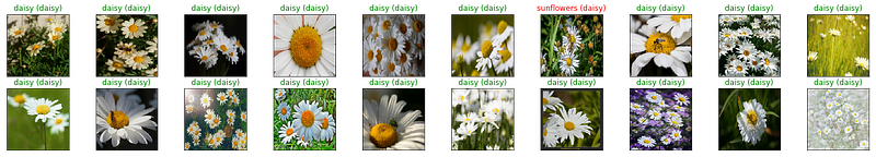
classes = ('daisy', 'dandelion', 'roses', 'sunflowers', 'tulips')Let’s visualize a few training images of our dataset.
dataiter = iter(train_loader)
images, labels = dataiter.next()
fig = plt.figure(figsize=(25, 4))
for idx in np.arange(20):
ax = fig.add_subplot(2, 10, idx+1, xticks=[], yticks=[])
plt.imshow(im_convert(images[idx]))
ax.set_title(classes[labels[idx].item()])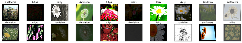
Step 6 : Instantiate the model
Now, we will use alexnet pre-trained network into our dataset.
model = models.alexnet(pretrained=True)
print(model)
After printing the Alexnet model, you will see the whole network as below:
AlexNet(
  (features): Sequential(
    (0): Conv2d(3, 64, kernel_size=(11, 11), stride=(4, 4), padding=(2, 2))
    (1): ReLU(inplace=True)
    (2): MaxPool2d(kernel_size=3, stride=2, padding=0, dilation=1, ceil_mode=False)
    (3): Conv2d(64, 192, kernel_size=(5, 5), stride=(1, 1), padding=(2, 2))
    (4): ReLU(inplace=True)
    (5): MaxPool2d(kernel_size=3, stride=2, padding=0, dilation=1, ceil_mode=False)
    (6): Conv2d(192, 384, kernel_size=(3, 3), stride=(1, 1), padding=(1, 1))
    (7): ReLU(inplace=True)
    (8): Conv2d(384, 256, kernel_size=(3, 3), stride=(1, 1), padding=(1, 1))
    (9): ReLU(inplace=True)
    (10): Conv2d(256, 256, kernel_size=(3, 3), stride=(1, 1), padding=(1, 1))
    (11): ReLU(inplace=True)
    (12): MaxPool2d(kernel_size=3, stride=2, padding=0, dilation=1, ceil_mode=False)
  )
  (avgpool): AdaptiveAvgPool2d(output_size=(6, 6))
  (classifier): Sequential(
    (0): Dropout(p=0.5, inplace=False)
    (1): Linear(in_features=9216, out_features=4096, bias=True)
    (2): ReLU(inplace=True)
    (3): Dropout(p=0.5, inplace=False)
    (4): Linear(in_features=4096, out_features=4096, bias=True)
    (5): ReLU(inplace=True)
    (6): Linear(in_features=4096, out_features=1000, bias=True)
  )
)
You can see the input and out features of the network by printing function.
print(model.classifier[6].in_features)
print(model.classifier[6].out_features)
In order to keep fixing the update of the feature part of the network, we can code below:
for param in model.features.parameters():
    param.requires_grad = False
As you know Alexnet is trained on the ImageNet dataset which has 1000 classes whereas we have 5 classes in our dataset. So we are changing the last fully connected layer as below:
import torch.nn as nn
n_inputs = model.classifier[6].in_features
last_layer = nn.Linear(n_inputs, len(classes))
model.classifier[6] = last_layer
model.to(device)
print(model.classifier[6].in_features)
print(model.classifier[6].out_features)
Step 7: Create a loss function and optimizer
Now we are going to set the loss function and optimizer. Here, we are using cross-entropy loss and adam optimizer. The performance of a classification model whose output is a probability value between 0 and 1 is measured by cross-entropy loss. Adam is a stochastic gradient descent technique that uses first and second-order moment estimation. Using exponential moving average, the approach determines the gradient’s 1st-order moment (the gradient mean) and 2nd-order moment (element-wise squared gradient) and corrects its bias. Learning rate times 1st-order moment divided by the square root of 2nd-order moment provides the final weight update.
criterion = nn.CrossEntropyLoss()
optimizer = torch.optim.Adam(model.parameters(), lr = learning_rate)
Step 8: Training the network
In order to train the network for our dataset, we need a forward pass and then we need to calculate the loss. After calculating loss, we will calculate gradients. After that, we will update the weights based on the computed gradients. We will also track the loss and accuracy so that we can draw a loss and accuracy graph.
# keep track of loss and accuracy
running_loss_history = []
running_corrects_history = []
val_running_loss_history = []
val_running_corrects_history = []
class_total = list(0. for i in range(5))
for e in range(epochs):
running_loss = 0.0
running_corrects = 0.0
val_running_loss = 0.0
val_running_corrects = 0.0 # train the model #
for inputs, labels in train_loader:
# Move the training data to the GPU inputs = inputs.to(device)
labels = labels.to(device) # forward propagation
outputs = model(inputs) # calculate the loss
loss = criterion(outputs, labels) # clear previous gradient computation
optimizer.zero_grad()
# backpropagate to compute gradients loss.backward() # update model weights
optimizer.step()
_, preds = torch.max(outputs, 1)
running_loss += loss.item()
running_corrects += torch.sum(preds == labels.data)
else:
with torch.no_grad():
for val_inputs, val_labels in val_loader:
val_inputs = val_inputs.to(device)
val_labels = val_labels.to(device)
val_outputs = model(val_inputs)
val_loss = criterion(val_outputs, val_labels)
_, val_preds = torch.max(val_outputs, 1)
val_running_loss += val_loss.item()
val_running_corrects += torch.sum(val_preds == val_labels.data)
epoch_loss = running_loss/len(train_loader.dataset)
epoch_acc = running_corrects.float()/ len(train_loader.dataset)
running_loss_history.append(epoch_loss)
running_corrects_history.append(epoch_acc)
val_epoch_loss = val_running_loss/len(val_loader.dataset)
val_epoch_acc = val_running_corrects.float()/ len(val_loader.dataset)
val_running_loss_history.append(val_epoch_loss)
val_running_corrects_history.append(val_epoch_acc)
print('epoch :', (e+1))
print('training loss: {:.4f}, acc {:.4f} '.format(epoch_loss, epoch_acc.item()))
print('validation loss: {:.4f}, validation acc {:.4f} '.format(val_epoch_loss, val_epoch_acc.item()))Step 9: Predict the classes of all the test images
In this step, we will predict all the accuracy for all of our test images.
#Predicting the Category for all Test Images
#confusion_matrix
total_correct = 0
total_images = 0
confusion_matrix = np.zeros([5,5], int)
with torch.no_grad():
for data in val_loader:
images, labels = data
images = images.to(device)
labels = labels.to(device)
outputs = model(images)
_, predicted = torch.max(outputs.data, 1)
total_images += labels.size(0)
total_correct += (predicted == labels).sum().item()
for i, l in enumerate(labels):
confusion_matrix[l.item(), predicted[i].item()] += 1
model_accuracy = total_correct / total_images * 100
print('Model accuracy on {0} test images: {1:.2f}%'.format(total_images, model_accuracy))We can see, we achieved 81.48% classification accuracy on our flower dataset.
Model accuracy on 540 test images: 81.48%Step 10: Class-wise accuracy for all test images and Confusion matrix
Some time, we need to calculate the accuracy for each class wise of our test data. We can easily find out the class-wise accuracy by using the flowing code.
#class_wise accuracy
print('{0:5s} : {1}'.format('Category','Accuracy'))
for i, r in enumerate(confusion_matrix):
    print('{0:5s} : {1:.1f}'.format(classes[i], r[i]/np.sum(r)*100))
We can see the category-wise accuracy of our model.
Category : Accuracy
daisy : 91.3
dandelion : 90.9
roses : 70.3
sunflowers : 72.3
tulips : 79.8
For confusion matrix plotting, we use the flowing code.
#plot confusion matrix
fig, ax = plt.subplots(1,1,figsize=(8,6))
ax.matshow(confusion_matrix, aspect='auto', vmin=0, vmax=1000, cmap=plt.get_cmap('Blues'))
plt.ylabel('Actual Category')
plt.yticks(range(5), classes)
plt.xlabel('Predicted Category')
plt.xticks(range(5), classes)
plt.show()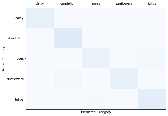
print('actual/pred'.ljust(16), end='')
for i,c in enumerate(classes):
print(c.ljust(10), end='')
print()
for i,r in enumerate(confusion_matrix):
print(classes[i].ljust(16), end='')
for idx, p in enumerate(r):
print(str(p).ljust(10), end='')
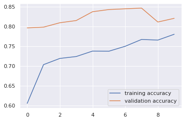
print()Step 11: Plot the training and validation loss and accuracy curve
We can use the flowing code for drawing the loss and accuracy curve during training our model.
import seaborn as sns
sns.set()

plt.plot(running_loss_history, label='training loss')
plt.plot(val_running_loss_history, label='validation loss')
plt.legend()
plt.plot(running_corrects_history, label='training accuracy')
plt.plot(val_running_corrects_history, label='validation accuracy')
plt.legend()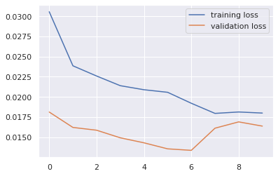
Step 12 (Optional): Classify an image from web
You can also classify an image from web using our deep neural network.
import PIL.ImageOps
import requests
from PIL import Image
url = 'https://images.homedepot-static.com/productImages/e350ef76-f7ff-46ee-83d2-606aab23453c/svn/mea-nursery-rose-bushes-62014-64_1000.jpg'
response = requests.get(url, stream = True)
img = Image.open(response.raw)
plt.imshow(img)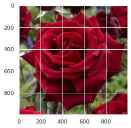
img = transform(img)
plt.imshow(im_convert(img))
image = img.to(device).unsqueeze(0)
output = model(image)
_, pred = torch.max(output, 1)
print(classes[pred.item()])Step 13 (Optional): Visualize the classification results with data
The following code is used to visualize the test results with ground truth classes and predicted classes.
dataiter = iter(val_loader)
images, labels = dataiter.next()
images = images.to(device)
labels = labels.to(device)
output = model(images)
_, preds = torch.max(output, 1)

fig = plt.figure(figsize=(25, 4))

for idx in np.arange(20):
  ax = fig.add_subplot(2, 10, idx+1, xticks=[], yticks=[])
  plt.imshow(im_convert(images[idx]))
  ax.set_title("{} ({})".format(str(classes[preds[idx].item()]), str(classes[labels[idx].item()])), color=("green" if preds[idx]==labels[id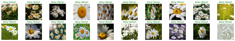
Find the full code here.
In this post, I show how can you classify your own dataset using a pre-trained network. Most of the time, we face the problem of small data set training using a deep neural network. We can overcome this issue using the transfer learning technique.
If you enjoyed my writing please consider sharing it around, following me on Facebook, Twitter, Youtube, or Instagram, or throwing some money into my tip jar on Ko-fi or Paypal. You can also support me by becoming a member on Medium for just $5 a month using my referral link:


