Chaos from the Logistic Map. Part 3: “Scrambled Sets (extended).”

This story intends to bring the construction of a ‘scrambled set’ that we started here to a conclusive end. The techniques we are going to use are once more taken from here and are mathematically not very sophisticated.

My intend is to make the text as readable as possible, but due to this environment’s lack of support for latex symbols, please apologize for making the following abbreviations:

f^k(x): denotes k-times composition of f, that is: f^3(x) f(f(f(x)))

A \intersect B:  means the intersection of the sets A and B

A \subset B:  means A is a subset of B

A \superset B: means A is a superset of B

A \union B: means the union of A and B

\empty: denotes the empty set

x \in B: means x is element of B

x \notin B: mean x is not element of B

In our previous story we arrived at an uncountable set S within a compact interval I such that for a function with certain mapping criteria we have for any distinct pair p, p' \in S,

lim sup_i |f^i(p) - f^i(p')| > 0

In other words, for a very large part of I, two points will have distinct iterates under f at arbitrary high levels. So, if we iterate f for various initial points in I, say 10,000 times, and then plotting the next 1000 iterates for all these points, we still very certainly have points that do not expose any regular pattern.

Our aim will be to show that S contains another uncountable set, that in addition to the above

lim inf_i |f^i(p) - f^i(p')| = 0

In other words, two points p and p' after arbitrary large iterations, will again deviate by a constant distance from each and will come arbitrary close to each other.

“This would make the chaos complete”.

First of all, let us repeat the requirements we impose onto f:

f maps the interval I onto itself ,and I can be separated into two intervals K, L such that

f(K) = L

f(L) = I = (K \union L)

f(a) = b

f(b) = c

f(c) = a

[------K------|-------L------]
a             b              c

If you remember what we did to ensure lim sup ... > 0, then it was all about ensuring iterates to map from time to time into K in order to gain a positive distance. This, in particular, only worked well because K is mapped back to L, and so ensures that we can follow-up. But how to ensure points are getting again arbitrary close and at the same time to get them distinct by a fixed distance?

The basic idea is contained in the following consideration:

By the intermediate value theorem, since f(b) = c and f(c) = a, there exists a point b_1 in (b, c) such that

f(b_1) = b

Moreover, by the same theorem, since f(b) = c and f(b_1) = b, there exists a_1 in [b, b_1) such that

f(a_1) = c

[---------|----|-----|---------]
a         b   a_1   b_1        c    

By exactly the same argument, we can find another interval

[a_2, b_2] \subset [a_1, b_1]

such that

f(b_2) = a_1

f(a_2) = b_1

[---------|----|----|------|-----|---------]
a         b   a_1  a_2    b_2   b_1        c

This can be repeated to yield a sequence of intervals

[a_1, b_1] \superset [a_2, b_2] \superset [a_3, b_3] \superset ...

where always f(a_{i+1}) = b_i and f(b_{i+1}) = b_i.

In other words, iterates of f map and interval [a_i, b_i] outwards until it is L.

The endpoints of this sequences do converge monotonically against endpoint of an interval [a', b'], that is,

a_i -> a' from below

b_i -> a' from above

Since the function f is assumed to be continuous, we have f(a') = b' and f(b') = a'. Moreover, this shows a' > b, something that becomes important soon.

Two key takeaways from the above construction:

1. With n getting larger, the wrapping of [a’, b’] by [a_n, b_n] becomes closer and closer. In particular, the lengths of the intervals [a_n, a’] and [b’, b_n] shrink to 0.

2. f^n([a_n, a'] \union [b', b_n]) \superset ([b, a'] \union [b', c]). This easily follows from using the intermediate value theorem and that f(a_{n+1}) = b_n, f(b_{n+1}) = a_n.

Therefore, if we ensure that for any point p \in S, some specific iterations under f move p into [b', b_n], then these points become from time to time arbitrary close on the long run. Moreover, since after n iterations [b', b_n] is mapped to something that contains [b, a'] and [b', c] we either can move to K or back to [b', b_n] (note, K \subset f([b', c] and [b', c] \subset f([b, a'])).

More in details, by making use of Theorem 2 here, we may find an interval Q_1 \subset L such that f(Q_1) = [b', b_n]. We know, after n iterations Q_1 is mapped to something containing [b, a'] and [b', c]. So, we may find another interval Q_2 \subset Q_1 such that f^{n+1}(Q_2) = K. Here we used K \subset f^{n+1}(Q_1. Alternatively, we may find a set Q'_2 \subset Q_1 such that f^{n+1}(Q'_2) = [b', b_n].

In other words, the first choice would ‘bring’ the image away from [b', c], and the second repeats the bubbling-up from [b', b_n] to [b, a'] \union [b', c].

Exactly this we can encode in terms of sequences as has been done here. We just have to ensure that on that one hand sequences infinitely often come together at the same index into a [b', b_n] for all possible n, and on the other hand they infinitely often become different by one being in K and the other in a [b', b_n].

There are many ways of achieving this. One is, by just enforcing all sequences to be in [b', b_n] (encoded by 0) when the index is of form n^3. Then it takes n steps to ‘bubble-up’ from this small interval, and then sequences either get back into [b', b_n] (encoded by 0) or move into K (encoded by 1).

To each sequence there is a unique decreasing series of compact intervals (Q_i)_i (see above) which intersection intersection determines a point p. The set of all these points shall be denoted by S and we have achieved the following:

For any p, p’ \in S

lim sup_n |f^n(p) —f^n(p’)| > 0

lim inf_n |f^n(p) — f^n(p’)| = 0

Moreover, like we did here we can make S containing no periodic points and only those that belong to sequences that a different infinitely often. It is not hard to see that S is then an uncountable set.

We see, although we had to do a little more detailed work than in the related predecessor stories, the final result is worth it.

Next, let us underpin all this with some numerical experiments. As already pointed out, the dynamical system generated by the logistic maps fulfills for certain parameters the above requirement. Especially, this takes place when it has periodic points of order 3 (see here).

We are going to consider the case r = 3.9, that is, our dynamical system is the following:

f(x) = 3.9 * x * (1 - x)

x_{n+1} = 3.9 * x_n * (1 - x_n)

By Newton’s method, that is converging quadratically in our case, we determine a point of period 3. That is, we solve f^3(x) — x = 0 with a starting point 0.4 and using 10^8 iterations (very exact!), to yield

p = 0.4487177531952602...

Next, let us plot the first 100 iterations starting at p:

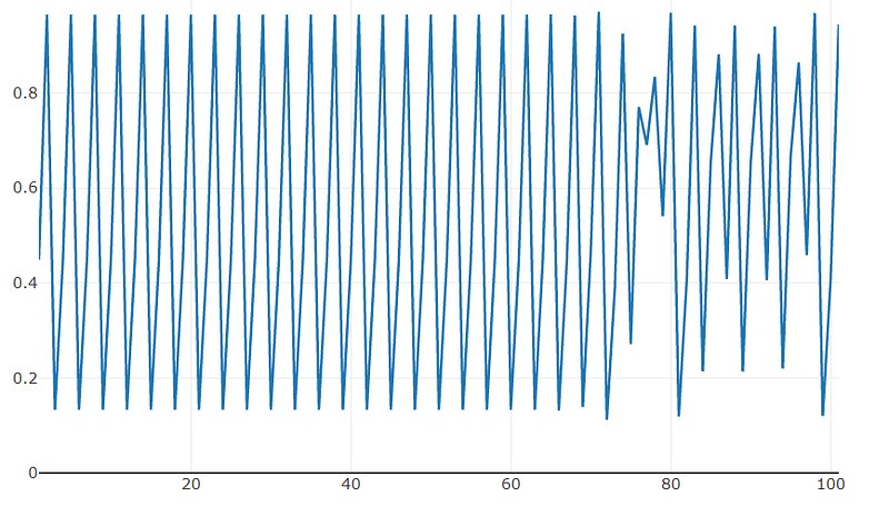
As we can see, only after 70 iterations, we leave the periodic behavior and enter a region where now clear pattern is observable. This is due to slight rounding errors that appear during the iterations have fatal influence on the qualitative behavior of the dynamics.

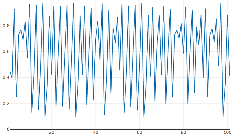
If we iterate the first 1000 steps starting with at p and then plot the the next 100 iterations the result becomes this:

Now let us compare how the situation changes when we start at a periodic point p_s that has a stable orbit. Such points have the property

For x chosen suitable near p_s

|f^k(x) - f^k(p_s)| < |x - p_s|    for all 0 < k </= n

where n is the order of the period.

This property says that starting with an initial value x near p_s, the iterations remain near to the hypothetical exact iterations at p_s.

For the logistic dynamics such a point exists for r = 3.627 at p_s = 0.4976878736755614 … that has a period of 6. For two initial points, one at p_s and the other at 0.53, we do like above 1000 iterations and then plot 100 further iterations. The result is this:

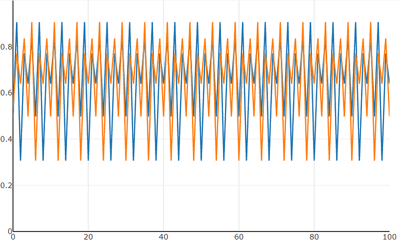
As you can see, the fact that the orbit is stable, makes the qualitative behavior of the system predictable near regions of p_s. I hope, these both examples make it a little bit clear what problems we are facing at chaotic regimes of dynamic systems.

This original inventors of above results shall gain all credit. You may find their original work here.

Thanks for reading!