Chaos from the Logistic Map. Part 1: “Periodic Points.”

The aim with this story is to present one of the most famous theorems in the research of chaotic maps. Before getting shrug-off too much, let me note early, this theorem is mathematically not more involved from what one learns in a first course of university level mathematics.

Throughout this account we will assume any considered map f to be a continuous real-valued function defined on some compact interval I. Moreover, we will assume f(I) \subset I. Therefore, we are able to build iterates like f^n(x), that denote n-times application of f onto the point x.

My intend is to make the text as readable as possible, but due to this environment’s lack of support for latex symbols, please apologize for making the following abbreviations:

f^k(x): denotes k-times composition of f, that is: f^3(x) f(f(f(x)))

A \intersect B:  means the intersection of the sets A and B

A \subset B:  means A is a subset of B

A \superset B: means A is a superset of B

A \union B: means the union of A and B

\empty: denotes the empty set

The two theorems stated below that are utilized in our argumentation do follow easily from the well known intermediate value theorem. So one could say, everything what is done here and in subsequent articles is an implication of this theorem!

Next, let us define what a periodic point is:

Definition (Periodic points)

A point p in I is called periodic with period k if

f^k(p) = p

f^i(p) != p for all 1 </= i < p

Periods are interesting to investigate for dynamic systems, that is, iterates of f, because some if these are stable. This in particular means that for points x sufficiently near to a stable periodic point p of period k, remain their distance after k iterations:

|f^k(x) - p| < |x - p|

In case a system f has only stable periodic points, we can focus our attention to these points in order to understand the system.

A criterion a map to have periodic points.

First we have the following theorem:

Theorem 1

If a map f: I -> I maps some interval J \subset I onto itself, that is,

J \subset f(J)

then there is some point p in J such that

f(p) = p

Such points usually are called fixed points and the above theorem is the 1-dimensional case of the fix-point theorem of Brouwer — but is way easier to prove for this case than for higher dimensions.

A criterion for a map f to have periods of order higher than 1 is a little more involved. For a period of k > 1, it basically must ensure that it maps a point p k-1 times into a point distinct from p and the k'th time exactly on p:

f^{i}(p) != p   for all i < k

f^{k}(p) = p

One way to ‘achieve’ this is by having two distinct intervals K and L in I

K \subset I

L \subset I

K \intersect L = \empty

[--|---K---|----|---L---|---]

and an interval Q \subset L such that

f^{i}(Q) \subset L       for i < k-1

So, the first k-1 iterations leaves Q in L and one further brings it to K:

f^{k-1}(Q) \subset K

Afterwards, yet another iteration brings it back to L:

L \subset f^{k}(Q) 

Then Theorem 1 would ensure f^k to have a point p in L with f^k(p) = p. This indeed must be a period of order k since for all other i </= k, f^i(p) cannot coincide with p, otherwise f^{k-1}(p) \subset K would not be possible.

Note, the above mapping could also be encoded as sequence of intervals that present the images under f:

L L L ... L L K L
 \         /
  k-2 times

Assertion

A map with the above ability would be one that maps K onto L and L back onto the interval K \union L:

L \subset f(K)

K \union L \subset f(L)

For this to see we utilize the following easy to proof theorem:

Theorem 2

Let U, V be closed intervals in I such that V \subset f(U), then there is an interval Q \subset U such that f(Q) = V.

In other words, we are able to find a subset Q in U such that f is meeting exactly the ‘target’ V.

As outlined above, the first k-2 iterations f should map to something that is contained in L and at the end is large enough to map onto K.

In L, since L \subset f(L), by Theorem 2, we may find an interval Q_1 such that

f^1(Q_1) = L

For the same reason, because f^2(Q_1) = f(L) \superset L, we may find another interval Q_2 \subset Q_1 such that

f^2(Q_2) = L

This way we can proceed to get a sequence of intervals

Q_1 \superset Q_2 \superset Q_3 \superset ... \superset Q_{k-2}

such that

f^{i}(Q_i) = L

Then since K \subset f(L), we find Q_{k-1} \subset Q_{k-2} with

f^{k-1}(Q_{k-1}) = K

And finally, because of L_2 \subset f(K), there is Q_k \subset Q_{k-1} with

f^{k}(Q_k) = L

This technique is a little like shooting the point p under iterates of f, but for the more iterates we want to dictate p landing in some region, the more we have to aim initially. The same technique can be used to find other interesting points that we are going consider in a later story.

Let us sum-up what has been shown above:

Theorem 3

A continuous map f: I -> I that is mapping two disjoint intervals L and K like

L \subset f(K)

K \union L \subset f(L)

has periodic points of all orders.

A map having periods of all orders already is quite an amazing feature. In particular, this means, since I is compact, the periodic points must accumulate somewhere. Therefore, there exists regions where we find arbitrary close points that have arbitrary different periods. So, to jump from a periodic orbit to another can be a matter of ‘millimeters’ and especially leads to fatal problems when it comes to computer-based simulations.

Logistic map:

A map that is famous for showing the above described behavior is the so called logistic map:

f: [0,1] -> [0,1]

x |-> r*x*(1-x)

with r in [0, 4]

This map arrives in so many applications (biology, chemistry, …) that it deems of highest interest to have a theoretical sound investigation — and very much has been done on this subject! We describe only a tiny but fundamental slice of this.

For different values of r we can consider roots within [0,1] of the algebraic equations

f(x) - x
f^2(x) - x
f^3(x) - x

to figure out where the dynamical system driven by f has points of period 3:

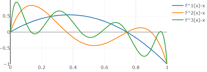
Points of period 3 are interesting in the context of this article because they imply the prerequisites of Theorem 3. This is again an application of the theorem of intermediate values:

Assume the periodic orbit is a < b < c with f(a) = b, f^2(a) = c, f^3(a) = a. In other words, f(a) = b, f(b) = c, f(c) = a. We can set K := [a,b] and L := [b, c] and see by the intermediate value theorem:

[b,c] \subset f([a,b])

[a, c] \subset f([b,c]) 

The graph above presents the typical shape for values of r over 3.9. A somewhat more interesting graph is the sometimes called bifurcation diagram:

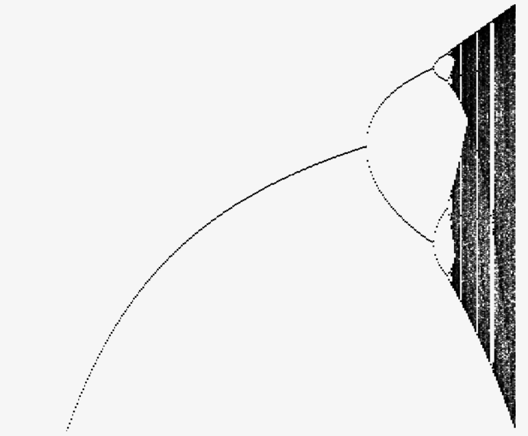
This shows for values of r in the range [0, 4] how the iterations evolve. This is, for a single r and some random x_0 in [0,1], we compute f^50,000(x_0), and then plot the last 1000 values of this iteration into the diagram (vertical axis). This we do for each value of r (horizontal axis).

The next simulation shows if we zoom into the area of [3, 4]:

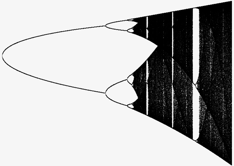
The regions at the left that display paths, belong to those where only a finite number of periodic points exists. The black regions indicate the applicability of the above theory, and we can be certain periodic points of all orders do exist. Actually, there is much more to say about these diagrams.

If you are interested in how to exactly produce such a bifurcation diagram with zooming functionality in Tauri/Rust, then let me refer you to this article.

Thanks for reading!