Cauchy’s Integral Formula

In my previous article (Contour integrals — a simple introduction) I discussed how to perform integrals of complex-valued functions in the complex plane, along a defined contour C by using techniques from line integrals on the real plane. In this article, we will look at slightly more complicated examples of contour integration in which the integrand contains a rational singularity, that is: there is some number z which makes the denominator zero.

Consider for instance the integral

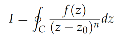
which is taken around some contour C. C is assumed to be a Jordan curve, meaning that it is closed and does not intersect itself at any point (examples of Jordan curves include circles, ellipses, etc.). This integral has a singularity (also known as a pole) at z = z0 if and only if z0 is enclosed within C. Suppose for instance, z0 = 3, but the curve C is a unit circle, then by definition |z|<1 meaning that z0 = 3 lies outside of C, and so it is not a singularity in that case.

Cauchy’s integral formula is stated as follows:

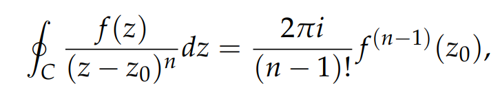
or more commonly

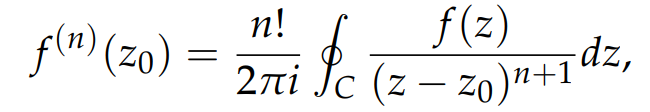
where the (n) superscript denotes the nth derivative of the function f(z), and it is evaluated at the point z=z0. Let us now look at a couple of examples.

Example 1

Evaluate the integral

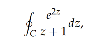
along the contour, C defined by |z| < 2.

Here, we look at the denominator and note how it is the same as writing (z+1)¹. The value which makes it zero is z = — 1, and this lies within |z| < 2 so we say it is a pole of order 1. Next, we look at the function in the numerator, which is

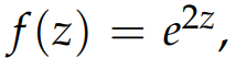
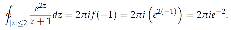
According to Equation 2, the integral evaluates to the (n-1)th derivative of f(z) where n is the order of the pole. Since this pole has order n = 1, the derivative will be the 0th derivative, which is basically the function itself, and therefore:

Example 2

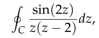
Integrate

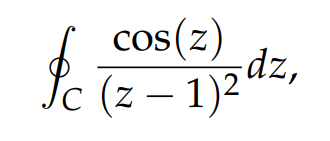
where C is defined by the circle |z| ≤ 3.

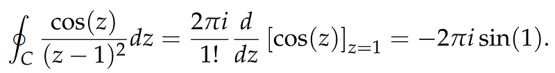
The contour encloses a single pole z = 1 of order n = 2. Therefore, by applying Equation 2 and using the fact that complex-valued functions follow the same differentiation rules and real-valued functions, we get

Example 3

Evaluate

where C is given by |z — 3| < 2.

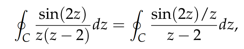
In this case, C is a circle of radius 2 centred at z = 3. Furthermore, there are two different poles for this function, one at z = 0 and one at z = 2, both which have order n = 1. The pole z = 0 does not lie within |z — 3| < 2, but z = 2 does. Because of this, the pole z = 0 can be moved into the numerator to create a new function:

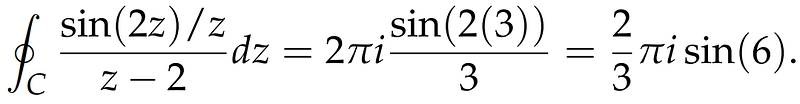
Then, we apply Cauchy’s integral formula to obtain

Example 4

Evaluate

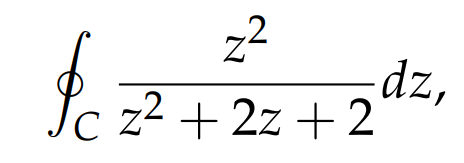
for C: |z| < 2.

The denominator is not in a form that is conducive to using Cauchy’s integral formula, therefore we must try and factorize it somehow. Using the quadratic formula, we find the following roots:

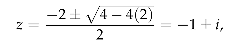
which means the following factorization is possible:

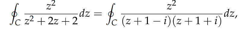
and looking at the modulus of each root we see that

both of which lie in |z| < 2. Because of this, we cannot use the same trick as we used in Example 3, because both poles contribute to the integral. Instead, we must separate this into a sum of integrals by applying the method of partial fractions. We start by writing

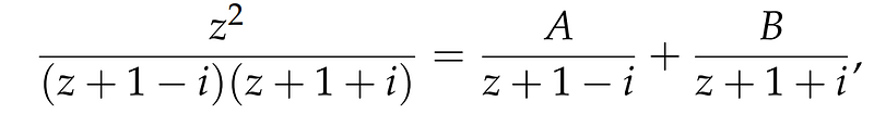
and multiplying both sides by the denominator of the LHS, we obtain

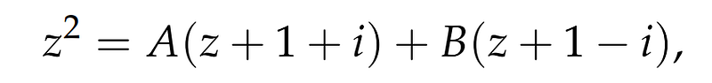
to find the coefficients A and B, we use the roots of z we found earlier. Starting with z1 = — 1 + i, we get:

Then, using z2 = — 1 — i, we get

and therefore the integral is split into two simpler ones:

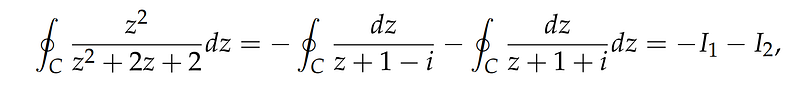
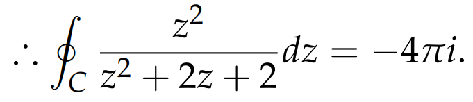
each of which is evaluated using Cauchy’s integral formula:

Example 5

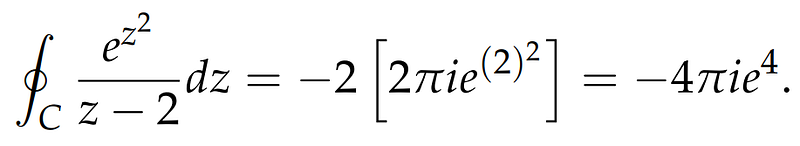
Our final example is the integral

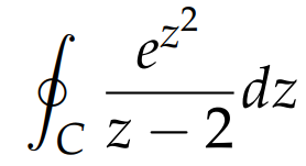
on an arbitrary contour C enclosing z = 2 twice in a clockwise manner. This one sounds a bit weird, so let’s unpack it: first, C is an arbitrary contour enclosing z = 2. What does that mean? It means C can have any shape, as long as it is a Jordan curve, so this does not affect the value of the integral. In fact, Cauchy’s integral formula implies precisely this: the value of the integral is independent of the shape of C and only relies on the poles enclosed within it. Second: the contour encloses z = 2 twice in a clockwise manner. By default, we use anti-clockwise orientation for contour integrals, but in this case, clockwise means we multiply the final answer by a negative sign. The fact that it goes around twice means that the integral will have 2 times the usual value (the number of times we traverse C becomes a multiple of the integral).

Hence, putting this all together and applying Cauchy’s integral formula gives us the final answer:

Cauchy’s integral formula is an extremely powerful tool used throughout applied mathematics, physics and engineering. Now that you know the basics, you can tackle a large variety of integrals.