Calculate Cost-Benefit in a Bayesian Knowledge Graph

Store data in Google Sheets, view the knowledge graph in Neo4j, and calculate cost-benefit with OpenMarkov

Currently, at least three pain points exist in the healthcare industry. Firstly, doctors may sometimes overlook certain potential causes for a set of symptoms, particularly in the case of rare diseases. As a result, this can lead to delayed diagnosis and potential misdiagnosis. Secondly, we are bad at probabilities. For example, smoking and obesity are often underestimated in terms of their harmful effects, whereas there is a tendency to overestimate the risks associated with rare types of cancer or genetic disorders. This can lead to either serious health consequences or unnecessary anxiety and stress. Thirdly, when it comes to making medical decisions that involve multiple factors and costs, we often struggle with making accurate and comprehensive cost-benefit calculations. As a consequence, patients may receive suboptimal care, and the healthcare system may become less efficient and effective in its delivery of services.

As mentioned in my previous article, How to Build a Bayesian Knowledge Graph, a Bayesian knowledge graph for healthcare can address the first two pain points. On the one hand, the knowledge graph in Neo4j can give both doctors and patients a comprehensive list of possible causes for a set of symptoms. On the other hand, the Bayesian inference with OpenMarkov can quickly calculate the odds of each possible cause based on the current evidence and prior knowledge. So doctors can focus on testing the most probable causes first, and patients can make informed decisions about each potential risk.

Thankfully, OpenMarkov has the capability to address the third concern as well. In fact, the cost-benefit analysis can be viewed as a practical application of Bayesian inference. And in this article, I want to build a Bayesian knowledge graph that depicts the medical choices for a suspected COVID-19 patient. OpenMarkov will generate various medical plans based on the patient’s preference for well-being and the prevalence of the disease (Figure 1).

The code for this project is hosted on my GitHub repository here.

The Google Sheets is here.

1. The use case

In this project, I have modified the use case from Chapter 5 in OpenMarkov’s tutorial, Multicriteria analysis with DANs and IDs. My data depicts the following fictional scenario: A citizen has COVID symptoms and goes to the hospital. The doctor needs to decide whether to test him and whether to do nothing or treat him with either Paxlovid or Remdesivir. The test and the drugs cost money. Each treatment (“Do nothing”, Paxlovid, and Remdesivir) has a different effect on his well-being. In my model, the well-being score is a proxy for effectiveness, and it ranges from 1 to 10. The higher the score, the better the treatment. Figure 2 shows the option trees.

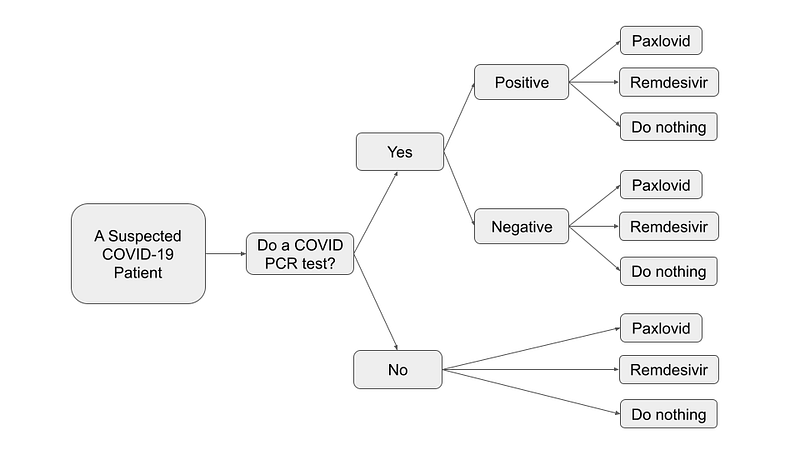
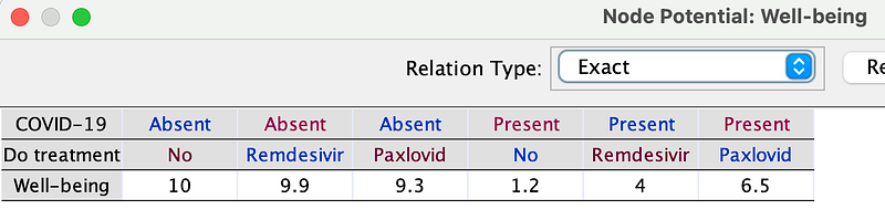
But the effect also depends on whether the citizen is really infected or not. In my COVID model, if the patient is not infected and does not undergo any treatment, his well-being score would remain at a perfect 10. However, if he opts for Paxlovid, his score would slightly decrease to 9.3. In contrast, if he is indeed infected, taking no action would result in a low score of 1.2, whereas taking Paxlovid could improve his condition and increase his well-being score to 6.5.

As you will see in the later texts, my Bayesian knowledge graph is going to capture this decision flow. With the help of OpenMarkov, we can personalize the plans based on the varying well-being valuations of individual patients.

2. The architecture

The software architecture in this project (Figure 3) is identical to that in my previous article. All the data are stored in Google Sheets. Neo4j again serves as our knowledge graph visualization platform. And OpenMarkov is our tool of choice for Bayesian inference and cost-benefit analysis. Different Python scripts channel the data between Google Sheets, OpenMarkov, and Neo4j.

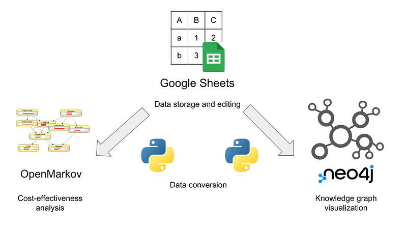
And Google Sheets is our single source of truth. That is, data changes in Google Sheets can be permanent. In contrast, OpenMarkov and Neo4j offer a sandbox where the user can freely explore various scenarios. If the user desires to save the changes back to Google Sheets, I have included some Python scripts for this purpose.

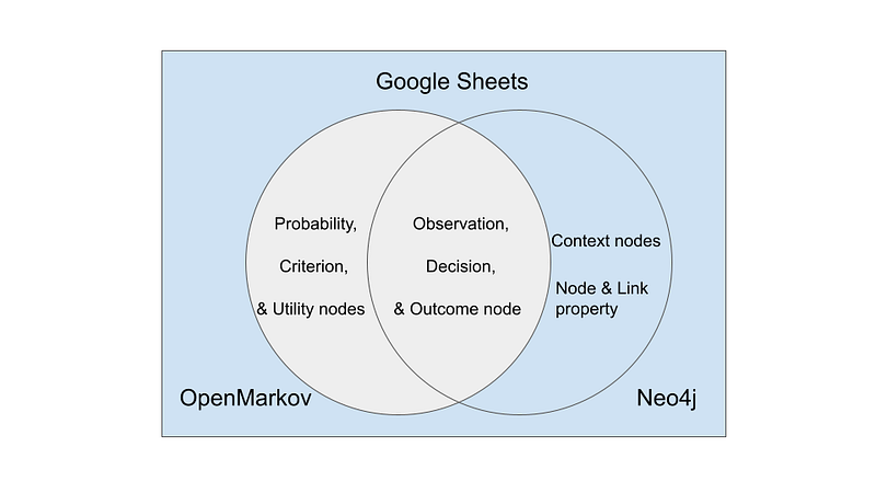
The reason for such a complicated setup is that no software on the market can manage knowledge graphs and cost-benefit analyses in one place. While they may have shared data, each application contains unique data that is not relevant or useful to the others. As shown in Figure 4, on the one hand, cost-benefit analysis requires probability tables, criteria, and utility nodes, which are not needed in the Neo4j visualization. On the other hand, the cost-benefit analysis only involves a subset of the complete knowledge graph. As a result, context nodes, information source nodes, as well as many node and link properties, such as IDs and descriptions, are not useful in the cost-benefit analysis. And we need Google Sheets to manage all this data.

3. Data in Google Sheets

All the links, criteria, probability, utility, and non-utility nodes are saved as separate tables in the Google Sheets.

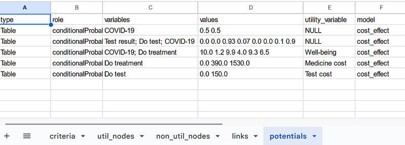
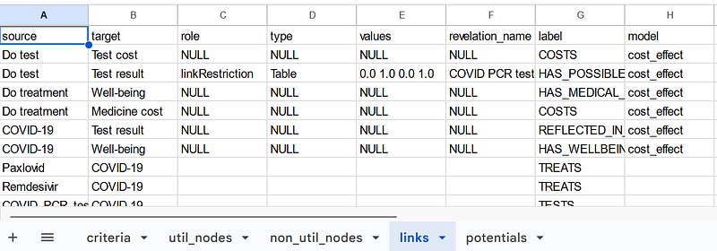
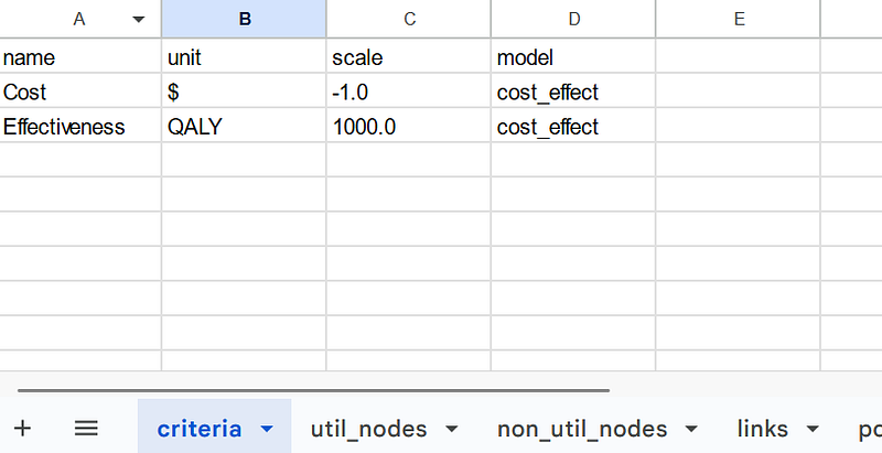
As I mentioned previously, the tables contain all the information for the cost-benefit analysis and the knowledge graph. In each table, the model property depicts to which model each data item belongs. The data items will be explained in detail in the next paragraphs.

4. Knowledge graph visualization in Neo4j

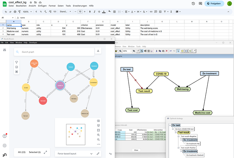
We can use the google_to_neo4j.py script to export all nodes and links from Google Sheets to Neo4j. In both Neo4j Browser and Bloom, we can easily examine the nodes, links, and their properties.

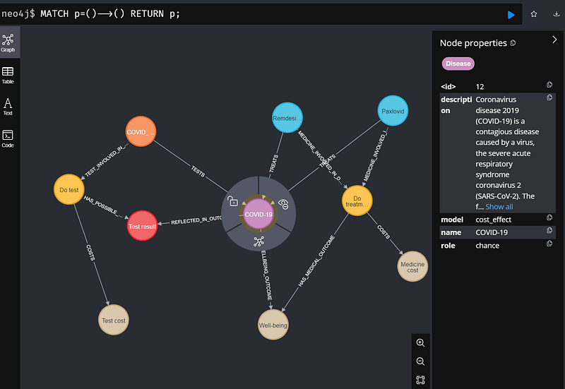
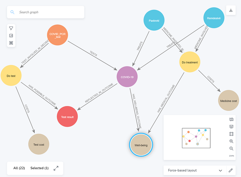
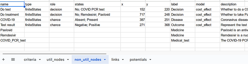
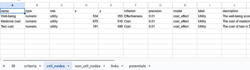
In this knowledge graph, we can see ordinary nodes that represent COVID-19, the drugs, the PCR test, the decisions, and the test result. But there are also three special nodes: Test cost, Well-being, and Medicine cost (tan in Figures 6 and 7). These are utility nodes that represent the cost and benefit of the medical decisions. They are unique to the cost-benefit analysis in OpenMarkov.

It is worth mentioning that three other nodes are not included in the cost-benefit analysis: COVID_PCR_test, and the two COVID-19 drugs Paxlovid and Remdesivir. They provide additional information and explanations pertaining to the medical concepts.

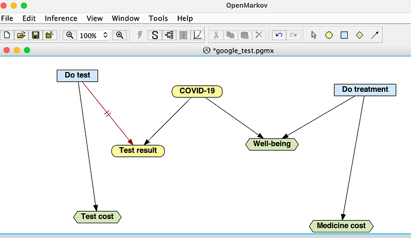
5. Cost-benefit analysis in OpenMarkov

Now, let’s do the cost-benefit analyses. First, use the google_to_pgmx.py script to export the data from Google Sheets as a PGMX file and open it with OpenMarkov (Figure 7).

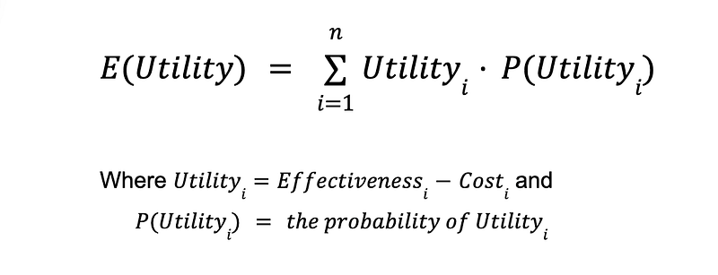
There are two types of analyses in OperMarkov. In the Unicriterion analysis, the patient first tells us how many dollars equate to one unit of effectiveness, i.e., his Willingness To Pay (WTP) for one unit of well-being. Once his WTP is known, we can convert effectiveness into a dollar value (hence the name Unicriterion) and then calculate the utility of a decision, which is its effectiveness minus the cost according to OpenMarkov.

If a decision may result in multiple possible outcomes with varying utilities, OpenMarkov can weighted-average the outcomes and calculate its expected utility E(Utility).

Unicriterion aims at determining the plan that maximizes the patient’s overall utility.

But putting a price on well-being is not always desirable. In this case, OpenMarkov can perform a second type of analysis called Cost-Effectiveness analysis, where effectiveness is not converted into money. OpenMarkov shows the effectiveness and cost separately for each scenario so that the user can decide the best option.

5.0 The model parameters

There are many parameters in the model and they all affect the results. I would like to fix some of them and leave the others as variables. It is important to note that the parameters used are approximations intended for illustrative purposes only.

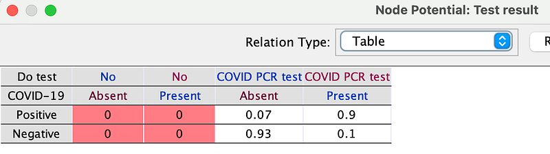
First, the PCR test has a sensitivity of 90% and a specificity of 93%. But if the doctor does not perform the test, there will be no result. And you can edit these data in the Test result node (Right-click ➡️ Edit probability …) in OpenMarkov.

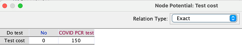
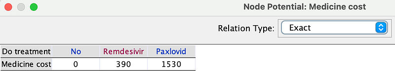
Second, the PCR test, Paxlovid, and Remdesivir are priced as follows. Similarly, you can edit them in the Test cost and Medicine cost nodes (Right-click ➡️ Edit utility …).

As mentioned above, the effects of the drugs also depend on whether the patient is infected or not (Figure 10). You can see them in the Well-being node (Right-click ➡️ Edit utility …).

Let’s calculate the different strategies for the following scenarios.

5.1 When COVID-19 is prevalent and the WTP is low, what is the best strategy?

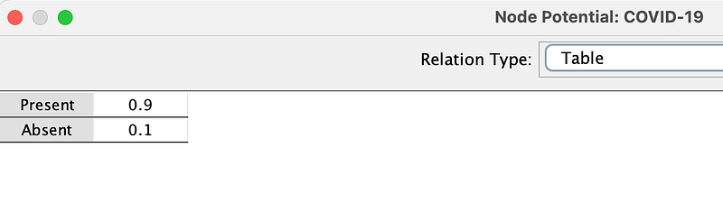
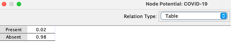
In the first scenario, the prevalence of COVID-19 is high (90%), as shown in the COVID-19 potential below.

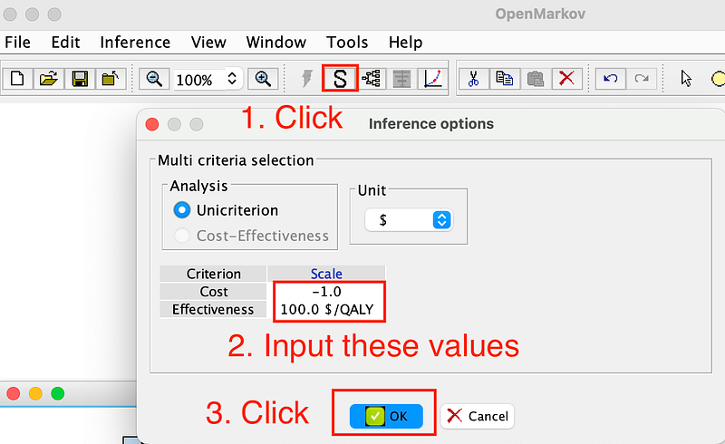
Meanwhile, the patient’s WTP is $100. To calculate the optimal strategy, click the Show optimal strategy button in the tool menu (Figure 12).

OpenMarkov shows the following decision tree (Figure 13).

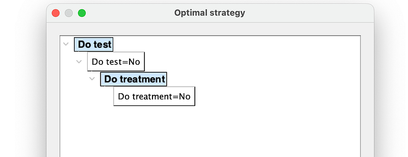
So for a patient with low well-being valuation, despite the high infection risk, it would be best for him to forgo both the test and the treatment.

5.2 When COVID-19 is rare and the patient values his well-being highly, what is the best strategy?

This is the converse of the previous scenario. Let’s change the COVID-19 potential and WTP as follows and re-run the analysis.

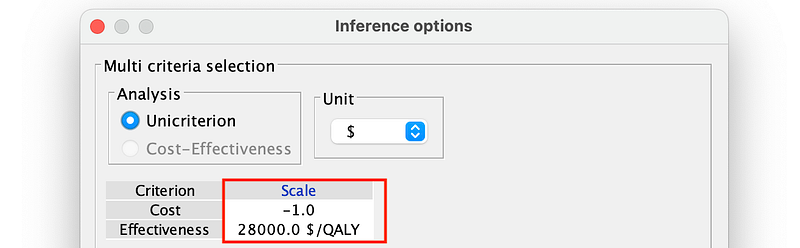
So the prevalence is 2% while the patient is willing to pay a high premium for his well-being ($28,000 per unit of well-being). And the best strategy is as follows (Figure 15).

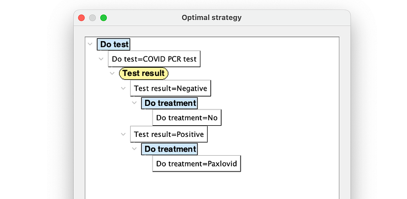
As you can see in Figure 15, the patient should first take the COVID PCR test. If the result is negative, he needs no treatment. But if the result is positive, he should take the more expensive Paxlovid.

5.3 When the risk of a COVID-19 infection is 50%, what are the strategies for different WTP?

In the last two analyses, only one optimal strategy could be generated for each WTP value. It would be nice if we can create the optimal strategies for different WTP brackets in one go. In OpenMarkov, this is called a deterministic analysis.

In this scenario, the COVID-19 prevalence is 50% (Figure 16).

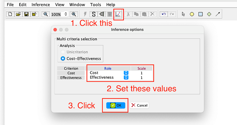
Then, click the Cost effectiveness analysis: Deterministic analysis button. Make sure that the values are the same as in Figure 17 and click OK twice to run the analysis.

And OpenMarkov will show the following result.

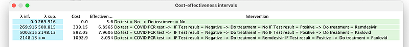
In this result table, λ sup. and λ sup. denote the lower and upper bounds of a WTP bracket. The last column Intervention describes the optimal policy for the given bracket. And the middle two columns show the cost and effectiveness of the strategy, respectively.

According to Figure 18, the best strategy for patients with low WTP (between 0 and 269.916) is to avoid both the testing and the treatment. This strategy costs them nothing. But their expected well-being is a mere 5.6. In comparison, patients in the next two brackets demonstrate a greater willingness to pay. They will do nothing if the tests are negative. Should they test positive, their treatment will involve the use of Remdesivir or the more expensive but more effective Paxlovid. As a result, they have higher expected well-being scores of 6.8 and 7.9. For the high-end patients in the last bracket, even if the test results are negative, it is recommended that they take Remdesivir as a precautionary measure because it has fewer adverse effects on the healthy body than Paxlovid.

Even though they are willing to pay top dollar for medicine, patients in the highest bracket have only a marginally higher expected well-being score (8.0) than those in the third bracket (7.9). But the differences between the first and the second, or between the second and the third bracket, are much more significant.

5.4 Cost-effectiveness analysis

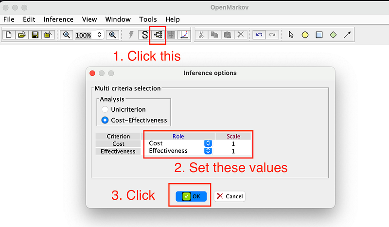
Finally, let’s set the COVID-19 prevalence to 86% and do a quick Cost-effectiveness analysis. You can start the process by following the instructions in Figure 19.

And OpenMarkov will then show you a full decision tree (Figure 20).

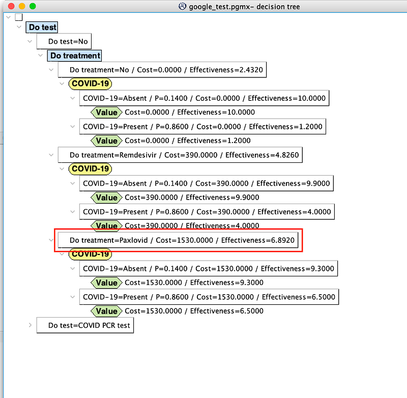
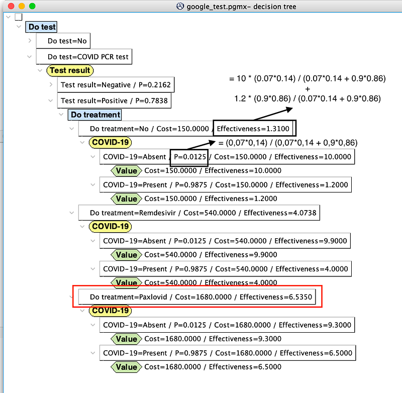
Remember that in a cost-effectiveness analysis, effectiveness is not converted into money. So in the decision tree above, we can see every single decision with its own cost and effectiveness. As stated at the beginning of Section 5, for decisions with multiple outcomes, OpenMarkov calculates their expected effectiveness. Based on this decision tree, doctors and patients can determine which intervention produces the highest effectiveness for a certain level of cost or which costs the least given the level of effectiveness. Or they can calculate the cost-effectiveness ratio and choose the plan that provides the greatest value for the investment.

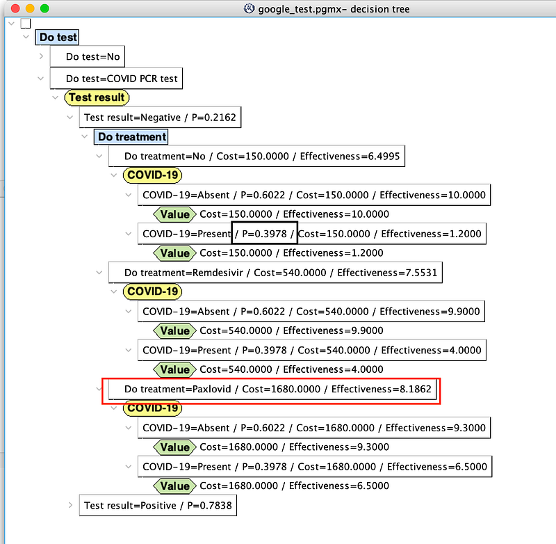
There are two interesting observations. Firstly, because the virus is so prevalent in this scenario, the patient still has a 40% chance of being infected even if his test result comes back negative (black rectangle in the middle section of Figure 20). This is an example of the so-called Medical Test Paradox. And it is a classical use case for Bayesian students, too.

Secondly, the high prevalence of COVID-19 favors the effective Paxlovid, despite being expensive and aggressive. It doesn’t matter whether the patient gets the test or what the test result may be, Paxlovid is always the most effective option. But due to its high cost, Paxlovid may be only accessible to high-end patients.

Conclusion

In healthcare, resources are limited, and the cost of treatments and interventions can be significant. So we need to make informed decisions and consider the cost and benefit of our medical choices. But the cost can be both direct (the cost of treatment or therapy) and indirect (lost productivity or quality of life). And the treatment benefits can be highly personal and multi-faceted. A mental cost-benefit analysis may prove inadequate, as there is a risk of overlooking important factors or making computational errors. In this case, a cost-benefit analysis within a medical knowledge graph can be of enormous help to doctors, patients, and insurance companies.

In this article, I have shown you how to build such a knowledge graph with Google Sheets, Neo4j, and OpenMarkov. The knowledge graph can present a comprehensive view of all the costs and benefits to the patients, providing them with a transparent understanding of the situation. The cost-benefit analyses allow them to compare the costs and outcomes of different options. As a consequence, they can identify the most cost-effective option and allocate resources accordingly. This knowledge graph can be applied to a wide range of decisions, from personal choices like purchasing a house to public decisions like building a new dam.

During the demonstrations, there are some noteworthy observations. And the one that struck me the most was in Section 5.1. Individuals who place a low value on their own well-being may choose not to undergo either testing or treatment. This population may be more likely to have lower incomes. They may have difficulties affording medical costs, and that can lead them to prioritize other expenses over healthcare. That is, they are “slipping through the cracks” of the social safety net. So it is essential for the healthcare system to provide fundamental medical services to the underprivileged population, especially during a pandemic.