Bitcoin’s Long Term Value

An Adoption S-Curve for a New Monetary Technology

This is not investment advice. Bitcoin is highly volatile. Past performance of back-tested models is no assurance of future performance. Only invest what you can afford to lose. You must decide how much of your investment capital you are willing to risk with Bitcoin. No warranties are expressed or implied.

*Figure 1: Technology adoption curves for some major inventions. Bitcoin is 12 years old and has 11% adoption in the US.*

Technology S-Curves

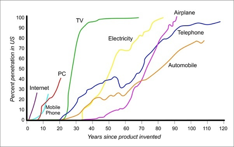
It is well known that technology adoption approximates an S-Curve or logistic function. It took half a century for electricity to be widely adopted in the US, a quarter of a century for half the population to get TVs, but mobile phone adoption took only half that time.

Bitcoin is still in its early adopter phase. This article estimates 11% of the population in the US own Bitcoin https://www.bitcoinmarketjournal.com/how-many-people-use-bitcoin/.

Bitcoin recently reached $1 trillion in market cap for the first time, but that is just a fraction of gold’s $10 trillion market cap. Bitcoin is often referred to as digital gold. Of course, gold has taken thousands of years to reach its present market cap.

It would be interesting to know if Bitcoin will reach gold’s total value ($10 trillion) or even exceed that level and begin to challenge the market cap of US equities ($50 trillion), 2/3 of which was accrued in the past decade. The value of all M2 broad money around the world is some $100 trillion. The US M2 total increased by 26% last year as the government and the Fed responded forcefully to the COVID crisis.

Many other models are not S-Curves

The best-known model for Bitcoin’s value is the stock-to-flow model, but it does not follow an S-curve. Rather it is a power law in market cap or price relative to the stock-to-flow (S2F), that is, in turn, an exponential with time, since S2F increases by a factor of 2 at each Halving separated by about four years. Folding these together results in effectively a very steep power law that is mathematically highly divergent. A couple more Halvings that will occur this decade would predict a price of order $10 million, implying $200 trillion of value, which is 2/3 of all wealth in the world, about the value of all real estate. One more Halving after that would imply a value exceeding all wealth in the world by nearly an order of magnitude.

So we need a better long-term model. Previously I introduced the Future Supply Model, that like the S2F model, depends on supply only, but in this case, on the integral of all not-yet-mined coins rather than the differential mining rate. It does not have an S-curve shape for market cap, rather a market cap that rises more slowly with time and asymptotes. It appears to be too conservative since it predicts an asymptotic value for Bitcoin’s market cap of around $1.6 trillion (in constant dollars), and we have already breached $1 trillion early this year.

I have also described a Lindy model that is a power law of block time, which uses the number of blocks laid down on the blockchain or the Block Years elapsed, which is the block height divided by 52,500. A Block Era between Halvings is four Block Years and has 210,000 blocks. block years are running about two weeks shorter than calendar years, on average.

It is very convenient to work in block years for calculation of stock-to-flow and of the fractional remaining supply of not-yet-mined Bitcoins.

A Lindy model has Price ~ Byr^k where Byr is block years elapsed and k is the power law index. A fit to prices yields an index k ~ 5.3, a steep power law. Like the S2F model, this is mathematically divergent, but much more slowly than S2F.

Weibull CDF S-curve model

The S-curve is often modeled with a logistic function. But there is a more general functional form of an S-curve known as the Weibull cumulative distribution function (CDF). It is characterized by three parameters: k a shape factor, c a characteristic time, and the saturation value (ultimate market cap, in constant dollars; think some percentage of global GDP or wealth).

The Weibull distribution has many uses in industrial and electrical engineering, weather forecasting, oil well production, survival analysis, and other applications. See the Wikipedia article Weibull distribution.

Here we model the market cap as a function of block years elapsed. The function looks like this:

f = 1 -exp [-(t/c)^k] ,

where f is the fraction of the maximum market cap (saturation) value reached by time t (in block years elapsed), c is the characteristic timescale, and k is the shape parameter. Note that for all k, f = 0.632 at time t = c.

Now for f << 1, when the adoption is relatively small, one can expand the exponential to first order and then f ~ (t/c)^k, and one recovers a power law form as a good approximation to the early adoption portion of the curve. We are arguably still in that early adoption portion. Thus it is not surprising that a Lindy model with a power law form gives a good fit.

Note that the power law fit referenced above for the Lindy model was analyzed in price terms, and here we are fitting to market cap. In fact, a power law model with regression of log market cap to log block year using the same data set yields a higher power law index of 5.96.

We use a Block monthly data set running from 2 block years elapsed to 12.75 block years elapsed for observed market cap values (12 block years marks the last Halving in mid-May, 2020).

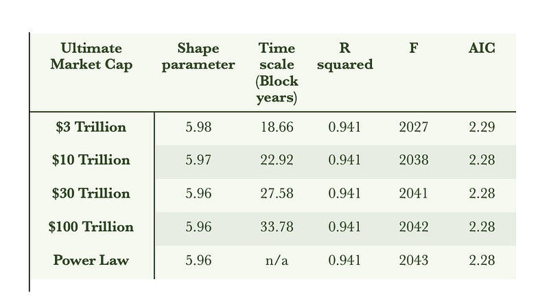
Since we have three parameters of ultimate market cap, time scale, and shape factor (essentially the power law index in the first portion of the curve), we run regressions for several different ultimate market cap values.

To run the regression one takes the log of both sides of the equation twice. One first puts in the form -ln (1-f) =(t/c)^k. Taking the log once more yields ln (-ln (1-f)) = k ln t -k ln c. One can then run a linear regression of the form y = a x + b by identifying y with ln (-ln (1-f)), the slope a with k, x with ln (t) and b with the last term. One recovers c with the relation c = exp(-b/k).

We have run the regressions using StatPlus for four values of the assumed ultimate market cap: $3 trillion (30% of gold’s market cap and more than in all government treasury vaults), $10 trillion (all gold), $30 trillion (60% of the value of all US equities), and $100 trillion (global M2 money supply). The results are in the table below:

*Table 1: Shape parameters and time scales, plus statistical parameters, for four ultimate market cap choices ranging from $3 trillion to $100 trillion*

A broad range of ultimate value still allowed

Examining Table 1, the conclusion is one cannot distinguish between the models. All have nearly the same R², rather good fits with 0.941 to three decimal places. All have F-values above 2000 and nearly identical Akaike information criteria values. The shape parameters are all about 5.96, corresponding to the power law fit applicable for early times. The good news is that it is just too soon, and it seems Bitcoin has a long way to run in its climb to greater value.

What does differ between these similar models then is the time scale for each, and the saturation market cap (which should be interpreted in terms of present-day dollars). The higher ultimate market cap requires a longer time scale to approach. It turns out that a higher ultimate market cap model actually has a somewhat lower fair value fit at present in the early portion of the S-curve, when compared to a lower ultimate market cap model.

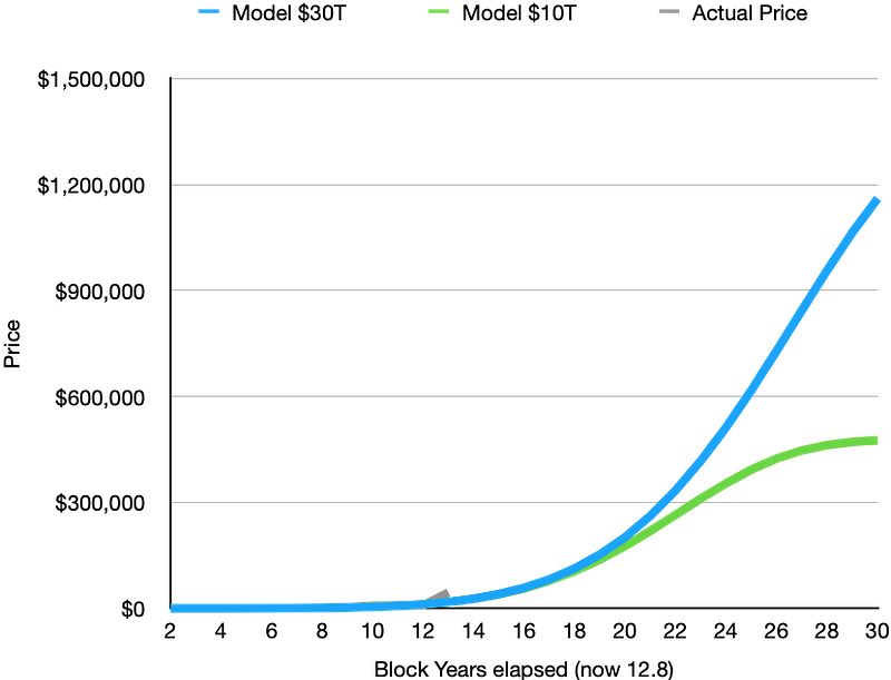
In Figure 2 below, we show the price curves for the prior 13 block years and fair value projections for the next 17 block years for the $10 trillion and $30 trillion ultimate value models. One can see the clear bend in the $10 trillion model as it heads toward a saturation price somewhat shy of $500,000. The $30 trillion model reaches 63% of its saturation value after 27.6 block years; one can see the flattening starting near the right edge of the chart. On this linear scale, the actual historical price curve is hardly distinguishable.

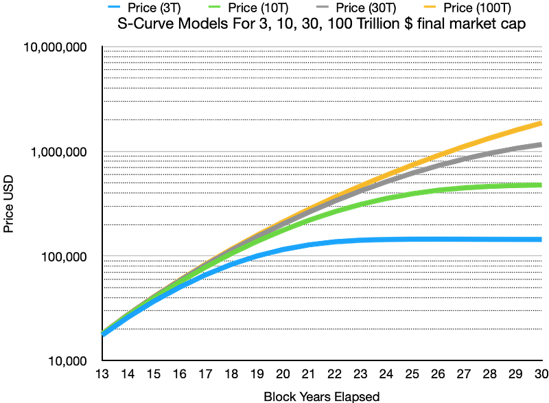
Figure 2: Bitcoin price curves (derived from market cap and supply vs. time) for a $10 trillion model and a $30 trillion model. Currently we are at 12.82 block years elapsed. Note that the $10 trillion model saturates 5% below $500,000 as expected, relatively soon after its 23 Block year timescale determined from the regression. The $30 trillion model is headed toward $1.43 million per Bitcoin, but is taking longer than 30 block years (17 years from now) to reach $1.2 million. The ordinate is linear in scale.

The next figure, figure 3, shows price curves for all four models on a logarithmic scale. The models are close to one another out to 15 or 16 block years but then begin to diverge significantly. The ultimate model fair value price projections are roughly $150,000, $500,000, $1.5 million, and $5 million, respectively.

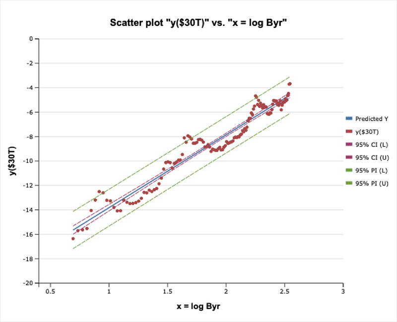
Figure 3: Bitcoin price curves (converted from fitted market caps vs. time) for $3 trillion, $10 trillion, $30 trillion, and $100 trillion models respectively. The price scale for the ordinate is logarithmic. The models are closely similar until block year 15 (2.2 years from now) and then the lower final market cap models begin to diverge downward.

The last figure shows the details of the fit from StatPlus for the $30 trillion model. The transformed variable y = ln (-ln (1-f)) as described above is plotted against ln (block years elapsed). The green dashed lines show the 95% probability interval for the data.

Figure 4: Fit of block monthly historical data using StatPlus for the $30 trillion ultimate market cap model. Here the ordinate y is the ln (-ln (1-f)) transformation described in the text. Despite the transformation the price run ups around each Halving are clearly visible. The green dashed lines are the 95% confidence interval for the data relative to the best model fit. The red dashed lines reflect the model uncertainty.

Bitcoin is not yet a teenager

Bitcoin is not yet a teenager, for a couple of more months in block year terms or ten more months in calendar year terms. These next seven years until it reaches age 20 block years are critical to its maturation and to its potential for capturing an ever greater share of value of the world’s assets. We would expect by the end of that interval to have a good sense as to whether Bitcoin will eventually achieve the $1 million price point.

Check out our new platform 👉 https://thecapital.io/

https://twitter.com/thecapital_io