The Future Supply Model, Era 4

Bitcoin is on a Block calendar

Witness at crums.io: 0515d51a66480ff94b4bb274e1214e5419c3181af7d970b39ee66f096b7022ce

“The portion of the integral calculus, which properly belongs to any portion of the differential calculus, increases its power a hundred-fold” — Augustus De Morgan

(This is not investment advice. Bitcoin is highly volatile, as demonstrated below.)

Abstract

In a previous article, I introduced the Future Supply model, using quarterly data (https://link.medium.com/bvWOCqrXr6 ) spanning nine and a half Block years of data on quarterly intervals. For this article I have refined the analysis by using a full ten Block years of data on Block monthly intervals (of 4375 blocks each). There are 121 price points in the series, that begins at the end of the first two Block years and runs through the end of Block year 12, coincident with the third Halving.

The Future Supply model (FSM) uses a measure of outstanding Bitcoin supply (future supply or reserves) rather than the annualized production used in the well-known Stock-to-Flow model. With FSM, the market cap asymptotes to a maximal value; log of market cap is modeled as a linear function of the fraction of all Bitcoin not yet mined.

We also evaluate both the Stock-to-Flow (S2F) model and a log Price vs. log Block time model against the same price and supply data. When expressed in Block year terms, S2F (annualized, forward-looking) is a monotonic formula, with discontinuities at each Halving.

The FSM is based on a continuous monotonically decreasing function, the remaining supply or its fractional value (either can be used as the basis variable). The model is mathematically convergent by design.

The statistical tests performed favor both the FSM and a log price vs. log Block time model over the S2F model somewhat, but that model also provides a good fit to the ten years’ worth of historical monthly data.

By the start of the next decade, the Future Supply Model predicts a Bitcoin fair value price of around $50,000 in constant 2020 dollars, whereas the S2F model forecast is over $8 million. While all three models examined in this article provide acceptable backward-looking fits, one should be able to distinguish which one is clearly superior by mid-decade, say a year or two after the next Halving has occurred.

Block time is not Stochastic

Construction of models is simplified by using the Block temporal basis. Block time is a more fundamental basis vector for Bitcoin. It is the inherent-to-Bitcoin calendar and temporal system that Satoshi Nakamoto laid out. Neither Block time nor stock-to-flow fluctuate with a random component; one is a counting system and the other follows a precise formula.

There is not a stochastic process until one reverts to calendar time; the random fluctuations then arise due to varying block times. Thus when analyzing the price or market cap time series in Block calendar or Block height terms, there is no issue of spurious correlation of two stochastic processes. There is one stochastic process being regressed against a monotonic Block time basis variable, or transformation of that in the S2F case.

Mark Burger covers this in greater detail in a recent article https://link.medium.com/VUTUPLmQE6 subtitled “The Fall of Cointegration,” showing how the deterministic elements dominate in stock-to-flow when viewed in ordinary calendar time.

Fundamentals of the Bitcoin Calendar and Creation

Price each block or each Block month is more meaningful for analyzing scarcity-driven long term price trends. Bitcoin is created by the block. Miners are paid by the block.

Bitcoin creation and value is driven by three fundamental timescales inherent in the Nakamoto consensus: the block, difficulty adjustments, and Halvings. These are the linchpins of the Bitcoin calendar and accounting system. Bitcoin becomes proportionally scarcer with each new block, and the inflation rate is continually lowered as the outstanding supply increases.

Bitcoin creation becomes more or less difficult in terms of miners’ compute power (hashrate) each Block fortnight (2016 blocks) as difficulty is adjusted upward or downward (upward, generally). Except for occasional miner shake outs with Halvings or sudden price drops, difficulty trends strongly upward as a result of faster mining rigs, more rigs deployed, and greater efficiency in crypto mining operations. (See the Brutal Efficiency of Crypto Mining article.)

However at Halvings, the inflation rate immediately drops a factor of two by cutting the Block reward subsidy in half. This shock-to-flow occurs each four Block years (210,000 blocks).

We have just passed the third Bitcoin Halving on May 11, 2020 (May 12 in Asia) and entered the fourth Block Era. Twelve Block years have elapsed since Bitcoin’s inception in January, 2009 and we have begun Anno Satoshi 13, as measured with Block years of 52,500 blocks each.

Table 1 below enumerates values for stock-to-flow and the fraction of Bitcoin not yet mined, out to the middle of the century. Calendar years are based on recent Block years being shorter by about two weeks.

Stock-to-flow (forward-looking, annualized) is given by the formula 2^(E+2)-8 at Halvings, where E is the new Block era. It increases by one each year between Halvings. Stock-to-flow heads toward infinity (reaching it in 2140 when the block subsidy is eliminated) and future supply declines more and more slowly each Block era.

Three Models

Three models are examined herein: the Future Supply Model for market cap, the Stock-to-Flow (S2F) model, and a simple Price vs. Block time (PvB) model.

All three models employ two parameters. The PvB and S2F models are power law (log-log) relationships, however S2F is itself an exponential function of Block time, in the limit. The Future Supply model is a simple log-linear relationship that has the market cap rising to an asymptotic value.

It is worth noting that Stock-to-Flow (annualized) is a strict monotonic function with Halving jumps when expressed in Block calendar terms; thus it also acts as a transformed temporal variable. The future supply (reserves) also follow a strict monotonic schedule. In fact the future supply or reserve profile is more fundamental than S2F which is a (Block) temporal derivative of the remaining supply.

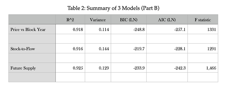
For each model, I determine best fit regression parameters (slope, intercept), R² values, standard error of the slopes (power law or exponential growth index), variance of observed values from model, and F-test and Bayesian information criteria values, using 121 data pairs. I also examine the residuals.

Future Supply Model

Does the market value for Bitcoin follow its annual inflation in supply (which is the inverse of stock-to-flow) or on the total outstanding supply? The integral or the derivative? One would have to say both in principle, certainly a fixed maximum supply of 21 million and a low (and declining) emission rate are both favorable to valuation. Here we explore whether a model based on all future supply can perform as well as or better than the S2F model.

If you had a gold mine, how would you value it? You would look at the reserves in place, and then estimate the cost of extraction, transportation, and refining. You would do a discounted cash flow analysis of this year’s production, and next year’s, and the year after that. You would go out into the future many years until the point at which you thought the remaining quality and quantity of reserves would make the mine uneconomic for further production based on your gold price forecasts, production cost inflation, interest rate forecast, and the like. And then you would add up all the discounted cash flows to arrive at a net present value of the gold mine.

If you had an oil field you would go through a similar analysis.

Bitcoin’s market cap valuation is not entirely different from this imperfect analogy. A model based on all future supply is analogous to the reserves of a mine with declining production. The S2F model considers declining production as well but accounts for only one year’s production. Now in the case of Bitcoin we as investors, traders, or HODLers do not care about what the mining costs were, we care about how it is valued relative to gold or the Euro or the US dollar or relative to other cryptocurrencies.

Crypto mining rigs are in a somewhat analogous situation as well. A given rig has a fixed hashrate but mining pools are continually adding new, faster equipment with better hashrate and higher efficiency of electrical power consumption. The Bitcoin produced by a single rig falls considerably over its lifetime. Whether the upfront capital cost and operating costs per rig (principally electricity) are recovered depends on the future behavior of mining difficulty and Bitcoin price.

What is different is that, unlike oil, there is no OPEC cartel to manage supply and unlike gold, there is no exploration and development of the reserves. Production will happen each block. Bitcoin production is inexorable. There is no traditional supply-demand curve, just a pre-determined new supply rate.

Until 2140 Bitcoin production never ceases, even in the face of an enormous crash in prices. It only slows in response to the algorithmically prescribed Halvings that drive the S2F parameter toward infinity. Any price crash will shut in much of the mining capacity, and if it persists the difficulty parameter of the Nakamoto consensus will adjust downward. The same number of Bitcoins will be mined regardless. In the short run, block times may lengthen or shorten in response to price fluctuations, the quasi-random nature of the cryptographic lottery, or miner behavior, but the Block fortnightly adjustments keep pushing the block time back toward ten minutes.

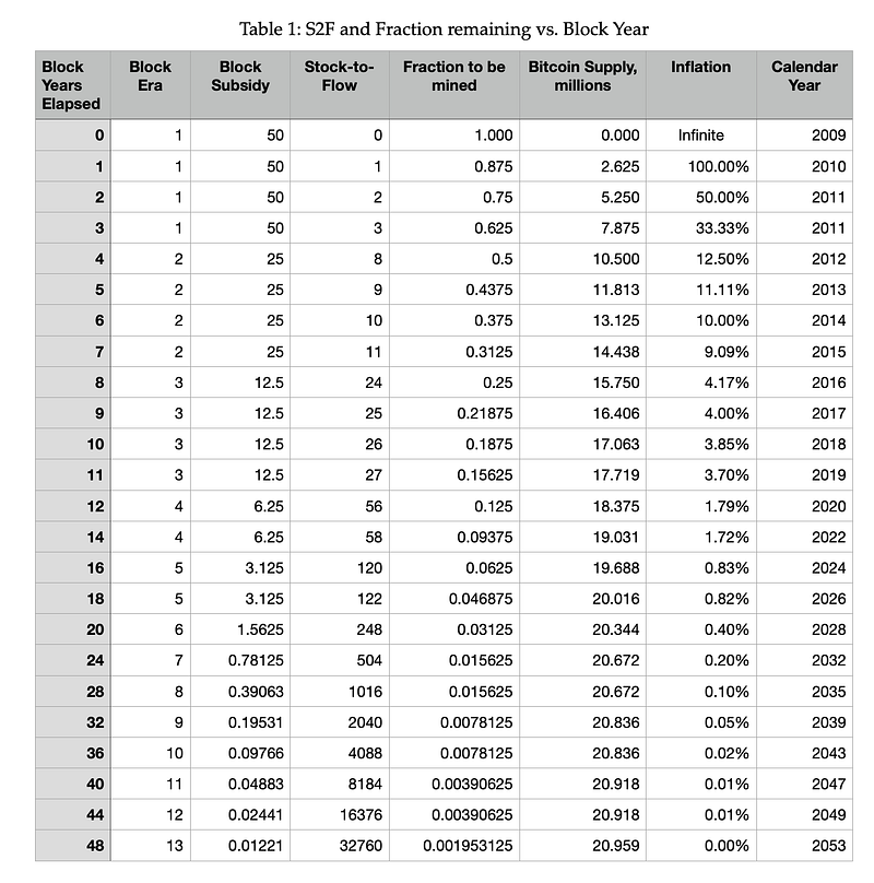
The Future Supply model is a scarcity model that is a function of only the remaining supply and yields a fit to an asymptotic market cap. It is explicitly designed to be convergent in the long-term, with a negative correlation between the remaining supply (of not yet minted Bitcoins) and the market cap. The market cap is modeled as log 10 (MC) = b + a*f, where f is the remaining fraction of 21 million Bitcoin yet to be mined, a is the slope (negative), and b is the asymptotic market cap.

When market cap is measured in billions of dollars, the best fit parameters are a = -7.15 and b = 3.16 corresponding to an ultimate market cap of $1435 billion (2020 dollars). The slope a can also be expressed in terms of millions of coins, in which case it is -0.34. This tells us that for a drop of a million coins in yet-to-be-mined supply the market cap of the model increases by a factor of 10^(0.34) = 2.19 times.

Compared to the fit in the first description of FSM with 9.5 years of Block quarterly data, the slope found has changed little, by about 2%. The asymptotic market cap has decreased by 12% relative to the $1628 billion found with the Block quarterly data and modeling.

The volatility relative to this model, as well as the others, is around a factor of two. For FSM the standard deviation is 0.355 dex or a factor of 2.26. The market cap could reach values 5.12 (2.26 squared) times larger or smaller than the forecast and still be at only two standard deviations removed.

How are the residuals distributed? We define a residual as positive if the log of the observed market cap exceeds the model. Of 121 residuals, 57 are positive, 64 negative. There are 20(25) observations greater than one positive (negative) standard deviation from the model, this is a bit more than expected for negative residuals. However there are 5(0) positive (negative) observations that are over two standard deviations removed.

Mark Burger (@BurgerCryptoAM) has noted the positive skew of Bitcoin returns in a May 18, 2020 tweet; with mean daily return over twice the median value. For this FSM the distribution is skewed negative around one standard deviation, but skewed positive around two standard deviations. One can see visually in Figure 1 that observed market caps hug the negative one standard deviation line but that three major price spikes pierce the positive one. This suggests that a Cauchy distribution for volatility would be a better description than a log-normal one, consistent with what Nick (@btconometrics) has just elucidated for Bitcoin’s upwardly biased daily return distribution.

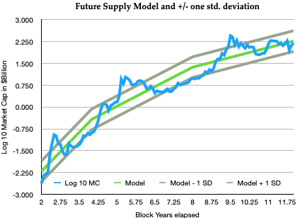
S2F Model

While FSM simply uses the entire remaining balance of Bitcoins yet to be mined, to establish its scarcity value (in current dollar terms), the S2F model is based on a derivative of that remaining supply, its issuance rate.

Various versions of PlanB’s S2F model have been released, using either price and market cap as the dependent variable.

The latest version is the Stock-to-Flow cross-asset model from PlanB. This model uses mean values of market cap and S2F in each Block era (although two ‘clusters’ in the first era) and adds silver and gold as beacons. (Only a single current value is used for each of gold and silver although Bitcoin is modeled as an evolving process).

PlanB’s best fit parameters for the cross-asset model are a power law index of 4.12 and an intercept of 12.76. The model predicts a typical price of $288,000 (market cap $5.5 trillion) during this new fourth Bitcoin era that has S2F = 56.

The S2F model effectively demands a continually steepening power law. This is because S2F itself grows as 2 to the power of the Block Era. Let E be Block Era, of duration 210,000 blocks (four Block years). We have just departed E = 3 and entered Era E = 4 on May 11, 2020.

As each new era begins, the forward-looking annual S2F = 2^(E+2)-8. You can check yourself that this formula yields 8 for the start of Block Era 2, yields 24 for the start of Block Era 3, and is 56 at the start of current E = 4. During a given era the S2F increases by one each Block Year, so there is a slow ramp and then an upward “shock to flow” at the Era boundary.

For large E, S2F ~ 2^(E+2). This approximation is accurate to better than 7% at E = 4 and 3.3% at E = 5.

Plan B’s S2F model looks approximately, for E > 3, like:

ln (MC) = b + a* ln (S2F) ~ b + a* ln [2^(E+2)] ~ b + 0.693 * a * (E+2)

Thus a power law in S2F model fit with index a is asymptotically a very steep power law in E with index ~ c * (E+2) and becomes steeper with each new block Era (here c = 0.693*a).

Plan B’s latest cross-asset model against gold has a = 4.12. At E = 4 this is roughly a 17th power of E model, and in four Block years with E = 5 it would need to steepen to a 20th power of E model (.69 x 4.12 x 7).

The steepness of this model, and its growing divergence, is troubling for the intermediate to longer-term and led me to formulate a convergent Future Supply Model.

I do not include a gold price point or silver price point in my own fit for S2F to the Block monthly data for two reasons. First, I want to compare the S2F regression to the FSM model with the same data set, on an equal statistical basis.

Second, adding gold to the S2F model pegs it (pushes it) toward a higher market cap value for large S2F. It begs the question being posed, biasing the model to behave in the assumed manner. This is especially true when also adopting the clustering strategy and combining all Bitcoin price and time observations into only four data points. That has the effect of increasing the weight of the gold and silver points considerably, so that they become one-third of the six resultant data points that are entered into the regression.

Our best fit parameters in this regression have a = 3.45 as the power law best fit, less steep than Plan B’s cross asset index value, and this results in a more modest $61,000 prediction for the model in 2022, with nearly a $1.2 trillion market cap two Block years from now.

The residuals of this article’s S2F model fit are quite differently distributed in comparison to those of the FSM. Exceeding the one standard deviation level there are 17 (20) positive (negative) observations. But at the two standard deviation level there are 0 (8) positive (negative) ones. One would expect 6 values at above two standard deviations; here they are all negative. Visual inspection of Figure 2 gives the impression of market cap trying to catch up to the model after each Halving, before piercing above, and settling back to the model region. That might be ameliorated by using a backward-looking (prior Block year) S2F.

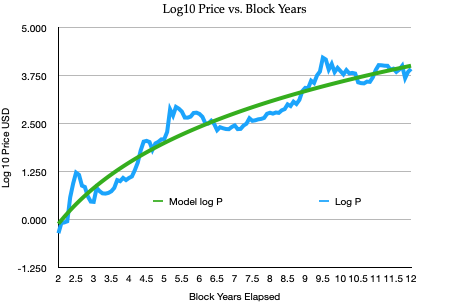
Price vs. Block Year model

This model is simply a power law of price against Block years elapsed, or log Price = b + a* log (Block years). It is the simplest Block temporal model that can provide a good fit. It does not explicitly consider Halvings, but their effect is realized implicitly. The model yields a power law index of a = 5.289, price ~ (Byr)^(5.29) where Byr is elapsed Block years. In other words, as the number of Block years elapsed doubles, the price rises by a factor of 39. This model appears to be the most statistically robust of the three with the best Bayesian information criteria and the lowest variance. However the FSM model has a higher R², lowest % error in its slope parameter, and higher F statistic.

The one standard deviation tails are 21 (20) for the positive (negative) side. But at two standard deviations all 7 of the values are skewed positive, consistent with visual inspection of Figure 3 below with 3 peaks that account for those 7 observations.

Of the three models, this PvB model is the easiest to compute since one does not need to calculate fraction of remaining supply or stock-to-flow or convert from market cap to price. But it also obscures the driving force of supply reduction, of scarcity. Supply reduction whether S2F increase or fraction of unmined supply decreases are then implicit influences (hidden variables) due to the progression of Block height.

Comparison of Three Models

A summary of the three models’ best fit parameters for slope and intercept and their statistical parameters are found in Table 2. In Part A, we also show the error in the slope and the standard deviation of the residuals between the observed price or market cap (in log base 10 terms) from the model best fit.

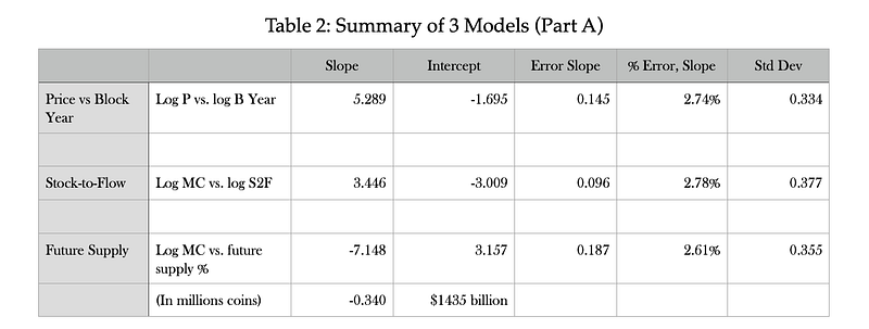
And in Part B of Table 2 we show the observed R² correlation, the variance and Bayesian and Akaike information criteria, as well as the F statistic. All models have very respectable fits to the ten years’ of Block monthly data. The R² values are not extremely high, around 0.92 for each model.

Long Term Price Forecasts

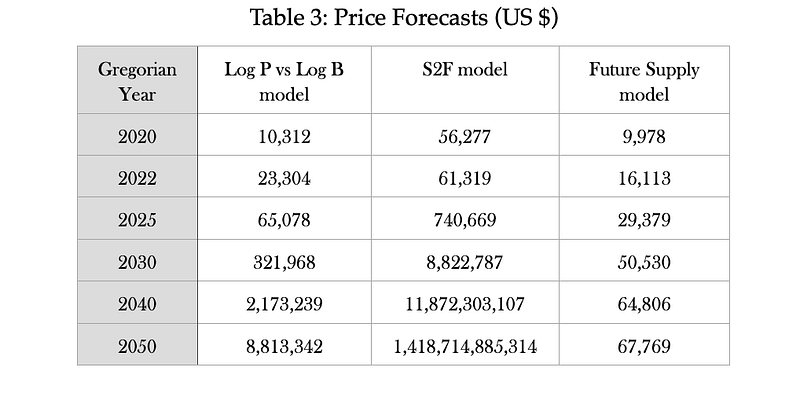
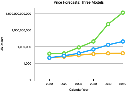
Using the best-fit parameters, we have calculated long term forecasts for the three models in Block years and then converted into Gregorian calendar terms assuming the two weeks shorter Block year compared to regular calendar year seen in recent years. For the S2F and Future Supply models that use market cap, the market cap forecast was converted to a price value based on the total Bitcoin supply at each future date. Table 3 has forecasts for 2020, 2022, 2025, 2030, 2040, and 2050.

The Price vs. Block year model and Future Supply model 2020 forecasts are near the current price, i.e. the current price is around fair value. The S2F model predicts a price that is higher by a factor of six. By 2025 the PvB model predicts around $65,000, the S2F model with the parameters found for this regression projects $740,000 and the FSM has the lowest target price of $29,000.

Because the price forecasts are very discordant, we should be able to discriminate in favor of one model, or at least rule out one of the models, by mid-decade. Although the volatility of Bitcoin is large, the FSM and S2F models differ by a factor of 25 in their mid-decade forecast; this is around four times the standard deviation of the Future Supply model.

HyperBitcoinization

HyperBitcoinization refers to Bitcoin becoming a major monetary asset to the point of driving out other monies. As two benchmarks, we have the US dollar M2 money supply at around $16 trillion and global M2 at around $90 trillion. The global amount of central bank gold is around $2 trillion (all gold $10 trillion). Given that the $, Euro, and Chinese Yuan have the largest money supplies, one might say hyperBitcoinization effectively arrives somewhere above the total valuation of central bank gold supplies and the M2 monetary supplies of Britain or Japan, the smallest two components of the IMF’s Special Drawing Rights. Then Bitcoin would join the top tier.

The Future Supply Model does not reach the market value of central bank gold with its centroid projection but that value is within the one standard deviation error range of the model. The model could accommodate a replacement of gold as the principal non-fiat reserve asset.

The PlanB model with S2F^(4.12) requires market cap to grow a factor of 17.4 for each additional Halving. This cannot persist for many more Halvings. Plan B’s model suggests $5.5 trillion is fair value for this era, and that would have to be followed one Halving later by roughly $95 trillion, which is equal to the global M2 money supply. Two Halvings later, by the end of this decade, the model would yield a market cap of order $1660 trillion. That exceeds all global wealth by a factor of over four and would require a Bitcoin price of roughly $80 million. That is well beyond even hyperBitcoinization’s wildest dreams.

There are at least a couple of ways hyperBitcoinization could happen. One is by excessive inflation and currency collapse in certain smaller national fiat currencies, so that sellers in those countries demand Bitcoin or other cryptocurrency (which they can exchange for Bitcoin). Usually the dollar plays that role for now. Another is by one or more central banks adding Bitcoin to strengthen its reserve position, alongside its gold and dollar and Euro reserves. This would most likely happen as part of a banking crisis, in a move to restore faith in the banking system and the national currency. The central bank in question would use Bitcoin for backing, probably fractionally, of its CBDC (central bank digital currency) and/or regular fiat.

We are facing ever greater monetary instability at present. Bitcoin’s rise and the Libra announcement sped up the exploration into CBDCs by a number of central banks; China is expected to roll out theirs, the DCEP, this year. The extreme fiscal and monetary policy measures causing previous unimaginable budget deficits and quantitative easing in response to COVID-19, together with the reality of a large number of looming corporate and personal bankruptcies, may trigger a monetary crisis; the Euro, in particular, is again facing much uncertainty around its future.

Summary

I have presented three two-parameter models for Bitcoin valuation with projections until the year 2050. Prices and supply, combined as market caps, and stock-to-flow and fractional supply remaining, were tabulated at each Block month boundary for the past ten Block years.

While all models fit the historical data well, both the FSM and Price vs. Block year model outperform the S2F model somewhat. All models reflect the high volatility of Bitcoin with standard deviations of over 0.3 dex, over a factor of two in linear price or market cap terms.

There is a large difference in the post-2030 price predictions, with the S2F model yielding extremely high price forecasts and FSM yielding lower price forecasts with a convergent market cap not very much above $1 trillion. The PvB model yields continued strong price rises, yet those are much more moderate than the S2F model.

Perhaps the 2010s were the decade of stock-to-flow valuation for Bitcoin. The 2020s could become an epoch of future supply valuation as that drops below one million Bitcoins remaining, and for the 2030s and beyond the narrative will be fixed quantity.

This is not investment advice. Bitcoin is highly volatile, as demonstrated above.