Bayesian Time Series Forecasting in Python with the Uber’s Orbit Package

An easy-to-follow guide of benchmarking Bayesian models to forecast univariate time series data

“The quest for certainty in forecasting outcomes can be the enemy of progress.” — Nate Silver

Time series forecasting makes predictions for future data and outcomes based on time-stamped past data collected over specified intervals of time.
Traditional time series forecasting methods rely on deterministic models to predict point forecasts as single-valued predictions of future values.
In contrast, Bayesian methods treat the model parameters as random variables with known prior distributions. Therefore, these methods quantify the uncertainty associated with the predictions.
Read more about Bayesian Structural Time Series (BSTS) vs ARIMA here [5].
In this post, we’ll walk through practical aspects of benchmarking Orbit for Bayesian time series forecasting, while utilizing probabilistic programming packages like PyStan and Uber’s own Pyro under the hood [1–4].
Orbit currently supports the the following forecasting models:

Exponential Smoothing (ETS), Damped Local Trend (DLT), and Local Global Trend (LGT).

Blog: Introducing Orbit, An Open Source Package for Time Series Inference and Forecasting GitHub: https://github.com/uber/orbit Documentation: Orbit’s Documentation Paper: Orbit: Probabilistic Forecast with Exponential Smoothing
Install Orbit from PyPi

!pip install orbit-ml

Applications

Orbit has a wide range of applications in Uber’s marketing data science team for measurement, planning, and forecasting. The latter is an important part of planning future marketing budgets and the optimization of spending across different channels and regions.

Grocery Store Sales Forecasting
Working with US Unemployment Benefits

Let’s delve into the aforementioned list of representative Orbit case studies to discover how analysts and data scientists from various industries can harness the power of Bayesian models.

Grocery Store Sales Forecasting

Input Store Sales Data

The Kaggle dataset will be used to predict sales for the thousands of product families sold at Favorita stores located in Ecuador. The training data includes dates, store and product information, whether that item was being promoted, as well as the sales numbers.
For the sake of simplicity, let’s use Orbit to process only one store [1].

Preparing Training/Validation Data

Importing libraries, reading the input dataset and selecting one store

import orbit
from orbit.models import DLT, ETS
from orbit.diagnostics.backtest import BackTester
import pandas as pd
import numpy as np

# Auxiliary WMAPE function


def wmape(y_true, y_pred):
    return np.abs(y_true - y_pred).sum() / np.abs(y_true).sum()

path = 'train.csv'
data = pd.read_csv(path, index_col='id', parse_dates=['date'])

# General data structure

data.tail()

          date   store_nbr item_nbr unit_sales onpromotion
id     
125497035 2017-08-15 54 2089339 4.0 False
125497036 2017-08-15 54 2106464 1.0 True
125497037 2017-08-15 54 2110456 192.0 False
125497038 2017-08-15 54 2113914 198.0 True
125497039 2017-08-15 54 2116416 2.0 False

data.info()

<class 'pandas.core.frame.DataFrame'>
Index: 125497040 entries, 0 to 125497039
Data columns (total 5 columns):
 #   Column       Dtype         
---  ------       -----         
 0   date         datetime64[ns]
 1   store_nbr    int64         
 2   item_nbr     int64         
 3   unit_sales   float64       
 4   onpromotion  object        
dtypes: datetime64[ns](1), float64(1), int64(2), object(1)
memory usage: 5.6+ GB

# Selecting store_nbr == 1

data2 = data.loc[((data['store_nbr'] == 1)), ['date', 'unit_sales', 'onpromotion']]

# Selecting training and validation sets


dec25 = list()
for year in range(2013,2017):
    dec18 = data2.loc[(data2['date'] == f'{year}-12-18')]
    dec25 += [{'date': pd.Timestamp(f'{year}-12-25'), 'unit_sales': dec18['unit_sales'].values[0], 'onpromotion': dec18['onpromotion'].values[0]}]
data2 = pd.concat([data2, pd.DataFrame(dec25)], ignore_index=True).sort_values('date')


train = data2.loc[data2['date'] < '2017-01-01']
valid = data2.loc[(data2['date'] >= '2017-01-01') & (data2['date'] < '2017-04-01')]

df_daily = train.set_index('date').resample('D')["unit_sales"].sum().to_frame()

df_daily.tail()

          unit_sales
date 
2016-12-27 12157.823
2016-12-28 12144.918
2016-12-29 10244.317
2016-12-30 13584.621
2016-12-31 10741.060

Training the ETS Model

Training the Bayesian Exponential Smoothing (ETS) model that makes use of prior knowledge in order to update their beliefs as new data becomes available.

ets = ETS(date_col='date', 
          response_col='unit_sales', 
          seasonality=7,
          prediction_percentiles=[5, 95],
          seed=1)

ets.fit(df=df_daily)

Making the ETS in-sample forecast for the training set and plotting the result

p = ets.predict(df=df_daily)

p.tail()

     date       prediction_5 prediction prediction_95
1455 2016-12-27 7802.727003 10143.287793 12110.888725
1456 2016-12-28 10014.508206 12579.779372 15058.306455
1457 2016-12-29 7358.604807 9569.571616 12158.040635
1458 2016-12-30 9646.606625 12375.098597 14963.530262
1459 2016-12-31 8467.247376 10494.881238 14305.702144

plt.figure(figsize=(15,6))
plt.plot(p['date'],p['prediction'])
plt.plot(p['date'],df_daily['unit_sales'])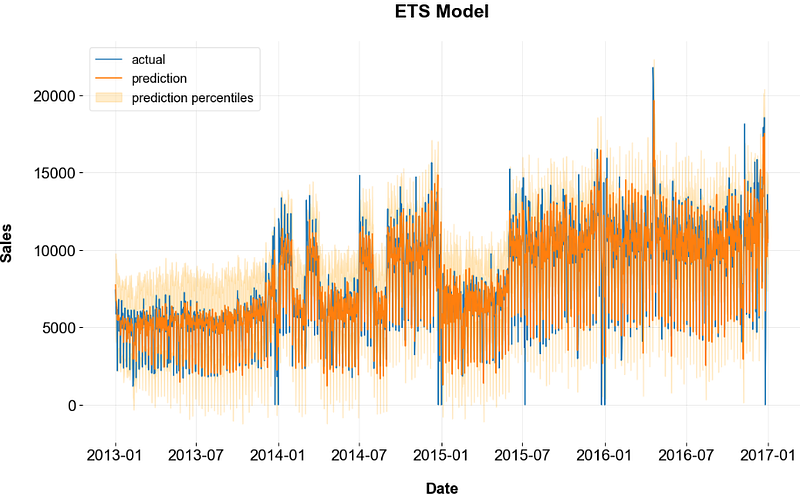

ETS Prediction & Percentiles vs Actual Training Data

Making the ETS out-of-sample forecast for the validation set and plotting the result

forecast_df = pd.DataFrame({"date": pd.date_range(start='2017-01-01', end='2017-03-31', freq='D')})
p = ets.predict(df=forecast_df)
p = p.merge(valid, on='date', how='left')

import matplotlib.pyplot as plt
fig, ax = plt.subplots(1,1, figsize=(1280/96, 720/96))
ax.plot(p['date'], p['sales'], label='actual')
ax.plot(p['date'], p['prediction'], label='prediction')
ax.fill_between(p['date'], p['prediction_5'], p['prediction_95'], alpha=0.2, color='orange', label='prediction percentiles')
ax.set_title('Error, Trend, Seasonality (ETS)')
ax.set_ylabel('Sales')
ax.set_xlabel('Date')
ax.legend()
plt.show()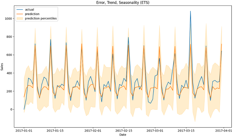

ETS Prediction & Percentiles vs Actual Validation Data

Training the DLT Model

Let’s look at the Damped Local Trend (DLT) Model. DLT is one of the main exponential smoothing models supported in Orbit. The model is a fusion between the classical ETS (Hyndman et. al., 2008)) with some refinement leveraging ideas from Rlgt (Smyl et al., 2019).
Training the DLT model with backtesting and checking various trend options by comparing their WMAPE scores

scores = dict()
for global_trend_option in ['linear', 'loglinear', 'flat', 'logistic']:
    dlt = DLT(date_col='date', 
            response_col='sales', 
            seasonality=7,
            prediction_percentiles=[5, 95],
            regressor_col=['onpromotion'],
            regressor_sign=['='],
            regression_penalty='auto_ridge',
            damped_factor=0.8,
            seed=2, # if you get errors due to less than zero values, try a different seed
            global_trend_option=global_trend_option,
            verbose=False)
    bt = BackTester(df=train, 
                    model=dlt, 
                    forecast_len=90,
                    n_splits=5,
                    window_type='rolling')

    bt.fit_predict()
    predicted_df=bt.get_predicted_df()

scores[global_trend_option] = wmape(predicted_df['actual'], predicted_df['prediction'])

print (scores)
{'logistic': 0.1870392532742924}

best_global_trend_option = min(scores, key=scores.get)
print (best_global_trend_option)
logistic

Preparing the trained data

df_daily = train.set_index('date').resample('D')["unit_sales"].sum().to_frame()

df_daily11 = train.set_index('date').resample('D')["onpromotion"].sum()

df_daily11.tail()

date
2016-12-27    259
2016-12-28    502
2016-12-29    258
2016-12-30    424
2016-12-31    252
Freq: D, Name: onpromotion, dtype: object


df_daily1.set_index('date')

df_daily1['date1'] = df_daily1['date']

df_daily1.set_index('date1')

df_daily = pd.concat([df_daily, df_daily1["onpromotion"]], axis=1)

df = df_daily.reset_index()

df.tail()

     date       unit_sales
1455 2016-12-27 12157.823
1456 2016-12-28 12144.918
1457 2016-12-29 10244.317
1458 2016-12-30 13584.621
1459 2016-12-31 10741.060

Fitting and predicting the trained data

dlt = DLT(
    response_col='unit_sales',
    date_col='date',
    estimator='stan-map',
    seasonality=52,
    seed=8888,
    global_trend_option='logistic',
    # for prediction uncertainty
    n_bootstrap_draws=1000,
)

dlt.fit(df)
p1 = dlt.predict(df)

p1.tail()

     date       prediction_5 prediction prediction_95
1455 2016-12-27 5459.263164 11730.18620 17904.642854
1456 2016-12-28 5672.749046 11715.39130 17625.631483
1457 2016-12-29 5819.880134 11716.52832 17927.297250
1458 2016-12-30 5553.716924 11625.78863 17753.949989
1459 2016-12-31 5770.091870 11692.68270 17509.058712

Plotting the trained data

fig, ax = plt.subplots(1,1, figsize=(1280/96, 720/96))
ax.plot(p1['date'], df['unit_sales'], label='actual')
ax.plot(p1['date'], p1['prediction'], label='prediction')
ax.fill_between(p1['date'], p1['prediction_5'], p1['prediction_95'], alpha=0.2, color='orange', label='prediction percentiles')
ax.set_title('DLT Model')
ax.set_ylabel('Sales')
ax.set_xlabel('Date')
ax.legend()
plt.show()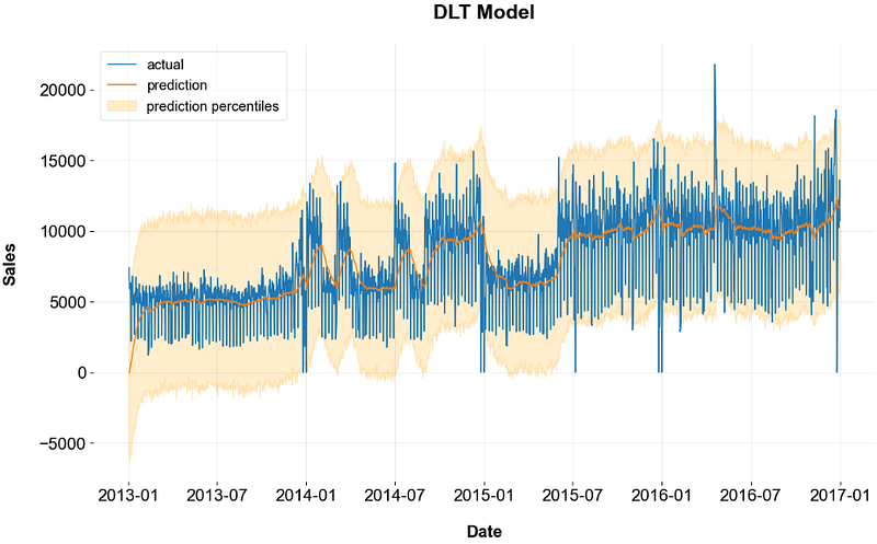

DLT Prediction & Percentiles vs Actual Training Data

Let’s train/fit the DLT model with the logistic trend and make predictions on the validation set

dlt = DLT(date_col='date', 
        response_col='sales', 
        seasonality=7,
        prediction_percentiles=[5, 95],
        regressor_col=['onpromotion'],
        regressor_sign=['='],
        regression_penalty='auto_ridge',
        damped_factor=0.8,
        seed=2, # if you get errors due to less than zero values, try a different seed
        global_trend_option=best_global_trend_option,
        verbose=False)

dlt.fit(df=train)

p = dlt.predict(df=valid[['date', 'onpromotion']])
p = p.merge(valid, on='date', how='left')

print(wmape(p['sales'], p['prediction']))

0.20177138495275543

fig, ax = plt.subplots(1,1, figsize=(1280/96, 720/96))
ax.plot(p['date'], p['sales'], label='actual')
ax.plot(p['date'], p['prediction'], label='prediction')
ax.fill_between(p['date'], p['prediction_5'], p['prediction_95'], alpha=0.2, color='orange', label='prediction percentiles')
ax.set_title('Damped Local Trend (DLT)')
ax.set_ylabel('Sales')
ax.set_xlabel('Date')
ax.legend()
plt.show()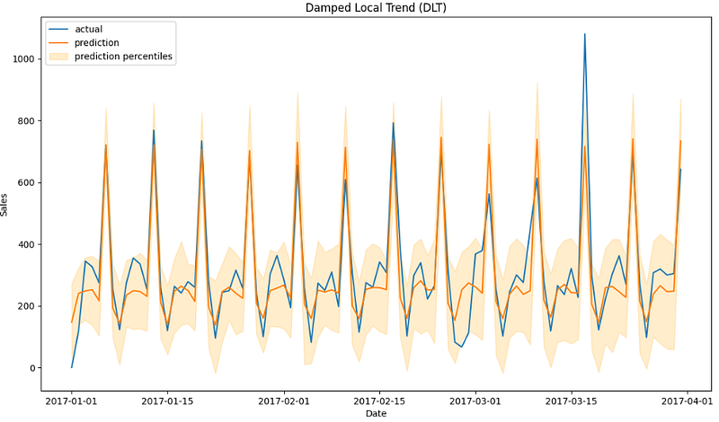

DLT Prediction & Percentiles vs Actual Validation Data

We can see a remarkable similarity between the ETS and DLT predictions on both training and validation sets.
It turns out that the KTR model yields the less accurate result (in terms of WMAPE) on the validation data

from orbit.models import KTR

ktr = KTR(date_col='date', 
        response_col='sales', 
        seasonality=[7, 28],
        prediction_percentiles=[5, 95],
        regressor_col=['onpromotion'],
        seed=2,
        verbose=False)

ktr.fit(df=train)

p = ktr.predict(df=valid[['date', 'onpromotion']])
p = p.merge(valid, on='date', how='left')

print(wmape(p['sales'], p['prediction']))

0.23352631577089197

Working with US Unemployment Benefits

Following the Orbit demo example, let’s address a forecast task on the iclaims dataset.
The iclaims data contains the weekly initial claims for US unemployment benefits against a few related google trend queries from Jan 2010 — June 2018. This aims to demo a similar dataset from the Bayesian Structural Time Series (BSTS) model (Scott and Varian 2014).
Importing the necessary Python libraries

import pandas as pd
import numpy as np
import orbit
import matplotlib.pyplot as plt

from orbit.utils.dataset import load_iclaims
from orbit.diagnostics.plot import plot_predicted_data, plot_predicted_components
from orbit.utils.plot import get_orbit_style
plt.style.use(get_orbit_style())
from orbit.models import ETS

orbit.__version__
'1.1.4.2'

Loading the log-log transformed weekly input data

raw_df = load_iclaims(transform=True)
raw_df.dtypes

week              datetime64[ns]
claims                   float64
trend.unemploy           float64
trend.filling            float64
trend.job                float64
sp500                    float64
vix                      float64
dtype: object

df = raw_df.copy()

df.head()

   week      claims    trend.unemploy trend.filling trend.job sp500     vix
0 2010-01-03 13.386595 0.219882           -0.318452 0.117500 -0.417633 0.122654
1 2010-01-10 13.624218 0.219882           -0.194838 0.168794 -0.425480 0.110445
2 2010-01-17 13.398741 0.236143           -0.292477 0.117500 -0.465229 0.532339
3 2010-01-24 13.137549 0.203353           -0.194838 0.106918 -0.481751 0.428645
4 2010-01-31 13.196760 0.134360           -0.242466 0.074483 -0.488929 0.487404

# Train/test data split

test_size=52

train_df=df[:-test_size]
test_df=df[-test_size:]

Training the ETS Model

Training, fitting the ETS model and predicting the train/test data

ets = ETS(
    response_col='claims',
    date_col='week',
    seasonality=52,
    seed=2020,
    estimator='stan-mcmc',
)

ets.fit(train_df)

predicted_df = ets.predict(df=df, decompose=True)
predicted_df

       week prediction_5 prediction prediction_95 trend_5 trend trend_95 seasonality_5 seasonality seasonality_95
0 2010-01-03 13.256093 13.386911 13.498341 12.922438 13.061019 13.179558 0.283892 0.324221 0.371806
1 2010-01-10 13.514679 13.625450 13.737572 12.959882 13.065062 13.158126 0.490289 0.562439 0.634173
2 2010-01-17 13.254438 13.382063 13.558862 12.943429 13.057401 13.205435 0.239650 0.324396 0.402475
3 2010-01-24 13.000500 13.158529 13.272095 12.917984 13.060074 13.169505 -0.006310 0.095894 0.171658
4 2010-01-31 13.052791 13.174475 13.322294 12.934345 13.077561 13.169154 0.017701 0.120735 0.213370
... ... ... ... ... ... ... ... ... ... ...
438 2018-05-27 12.119949 12.338702 12.548791 12.229486 12.443958 12.647680 -0.112899 -0.098516 -0.081082
439 2018-06-03 12.072402 12.280543 12.462557 12.238955 12.445619 12.640632 -0.183100 -0.169004 -0.147315
440 2018-06-10 12.147087 12.372973 12.578345 12.200795 12.442474 12.634412 -0.082059 -0.067508 -0.048729
441 2018-06-17 12.146767 12.328751 12.557206 12.239426 12.424625 12.657444 -0.112707 -0.097486 -0.077062
442 2018-06-24 12.183477 12.404675 12.562173 12.221322 12.457154 12.611574 -0.064576 -0.048535 -0.027940
443 rows × 10 columns

Plotting the above train/test data predictions vs actual data

_ = plot_predicted_data(training_actual_df=train_df,
                        predicted_df=predicted_df,
                        date_col='week',
                        actual_col='claims',
                        test_actual_df=test_df)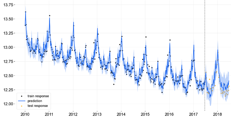

Train/test iclaims data vs ETS predictions

Plotting the predicted trend and seasonality components for the entire dataset

_ = plot_predicted_components(predicted_df=predicted_df, date_col='week')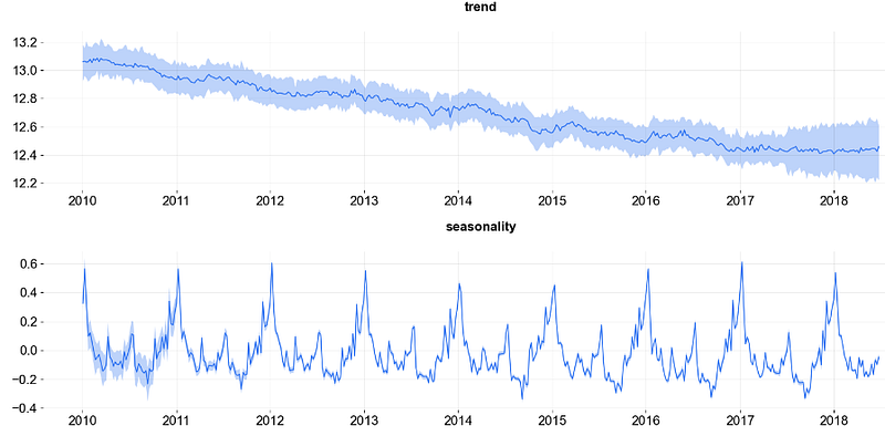

Predicted trend and seasonality components for the entire iclaims dataset

Analyzing the ETS posterior prediction samples

posterior_samples = ets.get_posterior_samples()
posterior_samples.keys()

dict_keys(['l', 'lev_sm', 'obs_sigma', 's', 'sea_sm', 'loglk'])

Posterior predictive checks (PPCs) are a great way to validate a model. The idea is to generate data from the model using parameters from draws from the posterior.
In doing so, we need a Python package for exploratory analysis of Bayesian models. ArviZ includes functions for posterior analysis, data storage, sample diagnostics, model checking, and comparison.
Installing ArviZ using pip

!pip install arviz

Plotting the ETS posterior samples “sea_sm”, “lev_sm”, and “obs_sigma”

import arviz as az

posterior_samples = ets.get_posterior_samples(permute=False)

# example from https://arviz-devs.github.io/arviz/index.html
az.style.use("arviz-darkgrid")
az.plot_pair(
    posterior_samples,
    var_names=["sea_sm", "lev_sm", "obs_sigma"],
    kind="kde",
    marginals=True,
    textsize=15,
)
plt.show()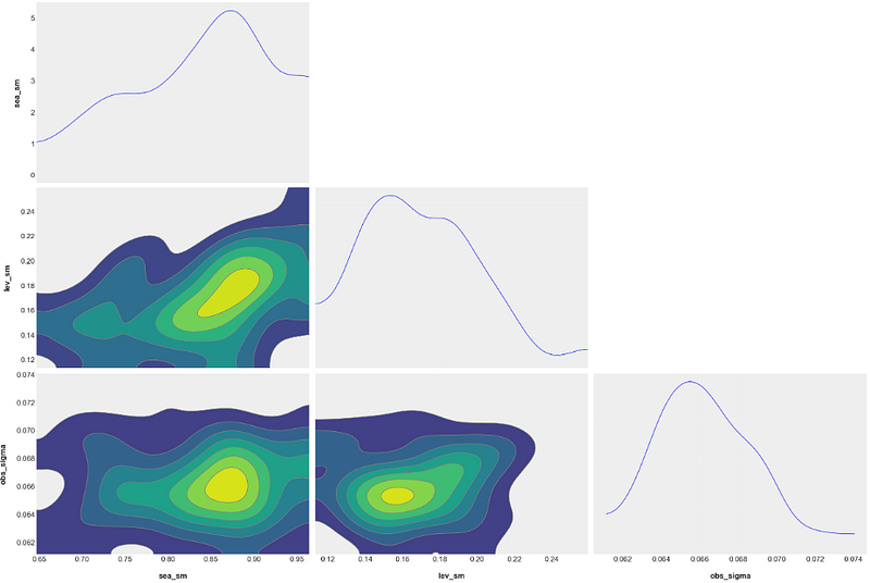

ETS posterior samples “sea_sm”, “lev_sm”, and “obs_sigma” as kde pair-plots

The above semi-unimodal distributions quantify the “uniqueness of fit”. That is, these probability density plots quantify how much model “ambiguity” there is when choosing from the possible interpretations.

Training the LGT Model

Let’s evaluate the Local Global Trend (LGT) model. It converts an additive log-transformed response into a multiplicative model with some advantages (Ng and Wang et al., 2020).
Specifically, the Orbit’s LGT model is a variant based on the multiplicative model proposed by Smyl in Rlgt. Its advantages over the original Rlgt models are two-fold: first, the computation is more effective with the additive form; second, in Rlgt is parameterized with that introduces dependency in noise generation, while is refined as an independent noise in LGT.
Importing libraries, loading the input dataset, train/test data split, training the LGT+MAP model and validating the LGT+MAP model predictions on test data

#Imports

import pandas as pd
import numpy as np
import matplotlib.pyplot as plt

import orbit
from orbit.models import LGT
from orbit.diagnostics.plot import plot_predicted_data
from orbit.diagnostics.plot import plot_predicted_components
from orbit.utils.dataset import load_iclaims

# load data
df = load_iclaims()
# define date and response column
date_col = 'week'
response_col = 'claims'
df.dtypes
test_size = 52
train_df = df[:-test_size]
test_df = df[-test_size:]

lgt = LGT(
    response_col=response_col,
    date_col=date_col,
    estimator='stan-map',
    seasonality=52,
    seed=8888,
)

lgt.fit(df=train_df)

predicted_df = lgt.predict(df=test_df)

_ = plot_predicted_data(training_actual_df=train_df, predicted_df=predicted_df,
                        date_col=date_col, actual_col=response_col,
                        test_actual_df=test_df, title='Prediction with LGTMAP Model')

Train/test response and prediction of test data with LGTMAP Model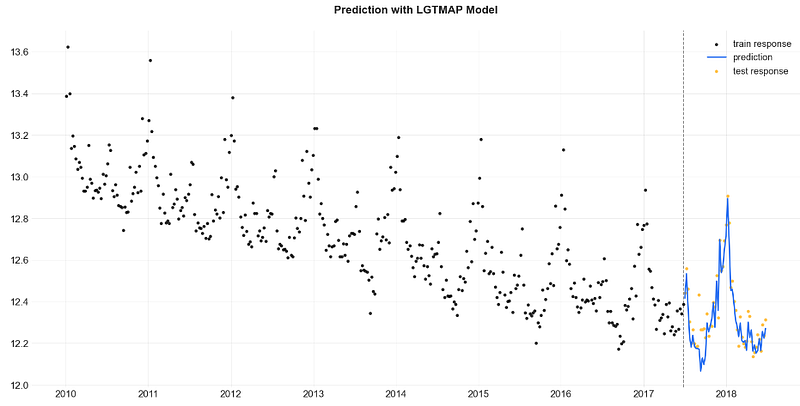

Training the LGT model with MCMC sampling (default) and validating the LGT+MCMC model (ref. LGTFull) predictions on test data

#LGT - MCMC
lgt = LGT(
    response_col=response_col,
    date_col=date_col,
    seasonality=52,
    seed=8888,
)

%%time
lgt.fit(df=train_df)

2023-12-03 15:57:45 - orbit - INFO - Sampling (PyStan) with chains: 4, cores: 8, temperature: 1.000, warmups (per chain): 225 and samples(per chain): 25.

CPU times: total: 281 ms
Wall time: 8.72 s
<orbit.forecaster.full_bayes.FullBayesianForecaster at 0x1f540348130>

predicted_df = lgt.predict(df=test_df)

predicted_df.tail(5)

   week     prediction_5 prediction prediction_95
47 2018-05-27 12.128395 12.218377 12.314531
48 2018-06-03 12.070700 12.171635 12.344855
49 2018-06-10 12.153305 12.278967 12.377019
50 2018-06-17 12.108882 12.239528 12.335686
51 2018-06-24 12.158394 12.278686 12.394868

lgt.get_posterior_samples().keys()

dict_keys(['l', 'b', 'lev_sm', 'slp_sm', 'obs_sigma', 'nu', 'lgt_sum', 'gt_pow', 'lt_coef', 'gt_coef', 's', 'sea_sm', 'loglk'])

_ = plot_predicted_data(training_actual_df=train_df, predicted_df=predicted_df,
                    date_col=lgt.date_col, actual_col=lgt.response_col,
                    test_actual_df=test_df, title='Prediction with LGTFull Model')

Train/test response and prediction of test data with LGTFull Model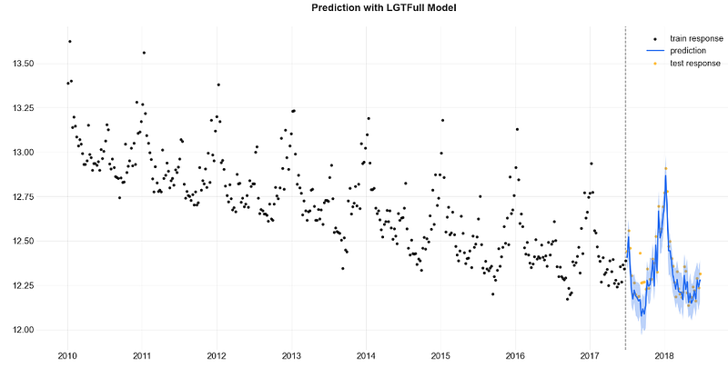

Training the LGT model with the mean point estimate method and validating the LGTAggregated model predictions on test data

#LGT - point estimate
lgt = LGT(
    response_col=response_col,
    date_col=date_col,
    seasonality=52,
    seed=8888,
)
lgt.fit(df=train_df, point_method='mean')

2023-12-03 16:05:48 - orbit - INFO - Sampling (PyStan) with chains: 4, cores: 8, temperature: 1.000, warmups (per chain): 225 and samples(per chain): 25.

predicted_df = lgt.predict(df=test_df)

_ = plot_predicted_data(training_actual_df=train_df, predicted_df=predicted_df,
                    date_col=lgt.date_col, actual_col=lgt.response_col,
                    test_actual_df=test_df, title='Prediction with LGTAggregated Model')

Train/test response and prediction of test data with LGTAggregated Model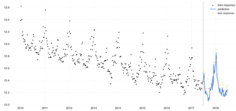

Observe a remarkable similarity between the LGTMAP and LGTFull model predictions on the test set.
Notice the least accurate LGTAggregated model predictions on the test set as compared to the LGTMAP and LGTFull validation results.

Training the DLT Regression Model

Let’s examine the DLT regression option of log-transformed iclaims data with the following obligatory settings

response_col = 'claims'
date_col = 'week'
regressor_col = ['trend.unemploy', 'trend.filling', 'trend.job']

Importing libraries, loading the input dataset, train/test set splitting, training the DLT model, and making in-sample predictions of the training set with decompose=True

%matplotlib inline

import pandas as pd
import numpy as np
import matplotlib.pyplot as plt

import orbit
from orbit.models import DLT
from orbit.diagnostics.plot import plot_predicted_data,plot_predicted_components
from orbit.utils.dataset import load_iclaims

import warnings
warnings.filterwarnings('ignore')
print(orbit.__version__)
1.1.4.2

# load log-transformed data
df = load_iclaims()
# train/test split
train_df = df[df['week'] < '2017-01-01']
test_df = df[df['week'] >= '2017-01-01']
# regression parameters
response_col = 'claims'
date_col = 'week'
regressor_col = ['trend.unemploy', 'trend.filling', 'trend.job']

#training the model

dlt = DLT(
    response_col=response_col,
    regressor_col=regressor_col,
    date_col=date_col,
    seasonality=52,
    prediction_percentiles=[5, 95],
)

dlt.fit(train_df)

2023-12-03 16:09:08 - orbit - INFO - Sampling (PyStan) with chains: 4, cores: 8, temperature: 1.000, warmups (per chain): 225 and samples(per chain): 25.

#making in-sample predictions of the training set

predicted_df = dlt.predict(df=train_df, decompose=True)

#plotting in-sample predictions of the training set

_ = plot_predicted_data(train_df, predicted_df,
                        date_col=dlt.date_col, actual_col=dlt.response_col)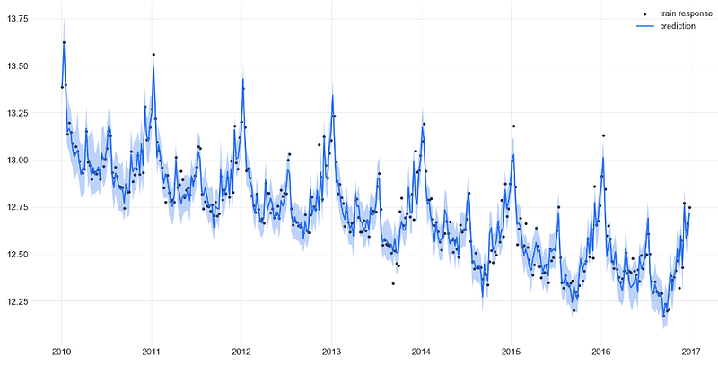

Training set vs in-sample prediction of DLT regression.

Applying the DLT regression to the test set and plotting the result

predicted_df = dlt.predict(df=test_df, decompose=True)

_ = plot_predicted_data(training_actual_df=train_df, predicted_df=predicted_df,
                        date_col=dlt.date_col, actual_col=dlt.response_col,
                        test_actual_df=test_df)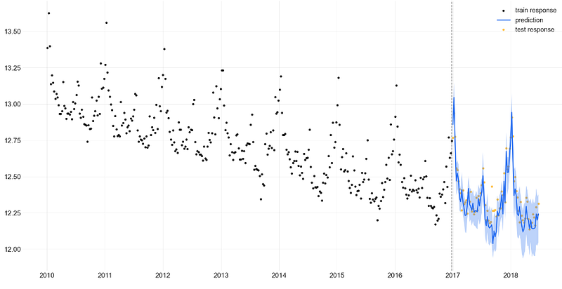

Training set vs out-of-sample test prediction of DLT regression

Plotting the key components vs error of DLT regression applied to the training set

predicted_df = dlt.predict(df=train_df, decompose=True)

_ = plot_predicted_components(predicted_df, date_col)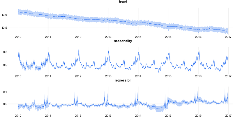

Trend, seasonality & error of DLT regression applied to the training set

Adding the training prediction result of DLT regression to the above plot

_ = plot_predicted_components(predicted_df, date_col,
                              plot_components=['prediction', 'trend', 'seasonality', 'regression'])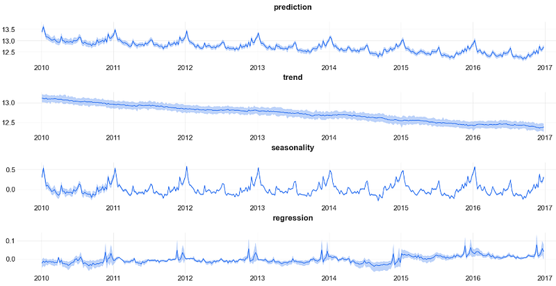

Prediction, trend, seasonality, and error of DLT regression applied to the training set.

Inferences:

Observe negligible errors of the DLT regression applied to the training set.
We can see a remarkable similarity between the LGTMAP, LGTFull model predictions and DLT regression (with acceptable 95% confidence intervals) on the test set.
The DLT decomposition unveils a significant downturn trend and a remarkable 1Y seasonal component.

Conclusions

Time series forecasting (TSF) is very important because it can be used to make informed decisions in a variety of industries and fields.
In this post, we have addressed the Bayesian TSF approach based on an assumption about the data’s patterns (prior probability), collecting evidence (e.g., new time series data), and continuously updating that assumption to form a posterior probability distribution.
Orbit is a general interface for the above approach used to conduct time series inferences and forecasting with structural Bayesian time series models for real-world cases.
As any other Bayesian TSF techniques, Orbit treats the model parameters as random variables with known prior distributions. Therefore, Orbit can quantify the uncertainty associated with the predictions.
We have shown that Orbit is the unique tool that allows for easy and accurate statistical modeling while not limiting itself to a small subset of models.
As with SARIMA and Prophet, Orbit enables the easy decomposition of a KPI time series into trend and seasonality components.
Overall, our two use cases of TSF have confirmed that Orbit can deliver robust end-to-end forecasting, provide explainability, quantify uncertainty, and perform a fast what-if scenario testing.

References

Explore More

Contacts

Disclaimer

The following disclaimer clarifies that the information provided in this article is for educational use only and should not be considered financial or investment advice.
The information provided does not take into account your individual financial situation, objectives, or risk tolerance.
Any investment decisions or actions you undertake are solely your responsibility.
You should independently evaluate the suitability of any investment based on your financial objectives, risk tolerance, and investment timeframe.
It is recommended to seek advice from a certified financial professional who can provide personalized guidance tailored to your specific needs.
The tools, data, content, and information offered are impersonal and not customized to meet the investment needs of any individual. As such, the tools, data, content, and information are provided solely for informational and educational purposes only.