An Introduction to Optimization For Convex Learning Problems in Machine Learning

In machine learning, we are often interested in better performance in our models. Therefore, there is forcedly a link between machine learning and the theory of optimization. In this article, we will explore optimization — specifically a few topics from gradient-based optimization. We also assume that we are working with a convex learning problem, i.e., that our function and hypothesis set is convex. It is assumed that this theory is known, else you start by reading the following article: Convex Learning Problems.

Understanding The Basic Definitions

Before we take the deep dive into understanding optimization, maybe we should first get a solid understanding of the basic definitions. As we can imagine, when we want to improve our model — what we are actually doing, is we are optimizing a function. Let us talk a bit more about this function.

Imagine that we have a function, f, which we can define like so:

Where we can say that:

Now, don’t worry about these notations. They simply mean that we have a function, which takes us from our set ‘M’ to the real line. In other words, the function takes something from a set as an input and outputs a number. Also, our set, M, is simply a subset of the space with d-dimensions. So, when we say that the space has d-dimensions it is like when we say that:

describes the 2-dimensional space. We have simply upgraded to having d-dimensions instead.

So, why are we interested in this function? Well, this will be our objective function. This is nothing more than the name to describe the function, which we want to either minimize or maximize. So we are either interested in maximizing:

or minimizing:

In our case, we are only interested in minimizing this function since it will often either be the function describing the error or risk of our model.

We can then also introduce some notation for when we have found the minimum. We can denote these points in the following way:

And these points also have a corresponding function value, the optimal value, which is denoted in the following way:

We can also call this the value of the optimization problem.

Now we are almost ready to finally get started. However, we remember that we focus on gradient-based optimization. Hence, we must forcedly assume that the objective function, f, is differentiable. The gradient is denoted in the following manner:

Constraint Optimization

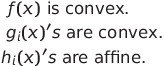
Let us finally get started with the optimization. We remember that we are only considering optimization for convex learning problems, which means that the objective function is a convex function and the solution set is a convex set. We will also later see how our problem being convex helps us later on when we consider the conditions for a minimum.

Firstly, we need to know how we can write our optimization problems in the standard form. Why? Because it will help us later on when we want to find the Lagrangian Function. The standard form is given by:

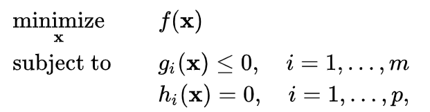
Where we have that:

Example of Finding Standard Form

We have now seen how the standard form looks for a convex optimization problem. Let us now try to take a few examples.

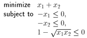
As a first example, let us imagine that we want to re-write an optimization problem into standard form. Imagine that we have the following problem:

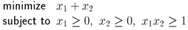
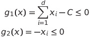
We can see that we have the following objective function and constraints:

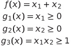
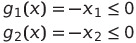
Hence we can see that we have no affine functions. We can then think about how we want to transform it into the standard form. We do not need to touch the objective function, only the constraints. So, the first two constraints are easy — we can simply write them like so:

We then look at the last constraint, we cannot simply write it like so:

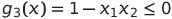
Why can we not? Since this function is not convex, which we need it to be! However, we can simply write it into:

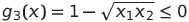
We have now made all our constraints into convex functions — so let us then see how our optimization problem would look on the standard form:

Hence, we have written our optimization problem on to the standard form. Not that hard was it? But for the sake of it, let us take another example.

Imagine that we have a convex optimization problem, which we want to write on the standard form. The problem is given by:

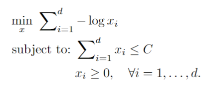
We then want to write onto the standard form. We can again consider what our objective function and the constraints are. We can see them here:

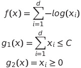
Again, we don’t need to touch the objective function — however, we need to change our constraints a bit such that they match the standard form. They become the following:

We can see that our constraints are convex functions. We can then see that our optimization problem becomes the following:

We have now written our optimization problem to the standard form.

Finding The Lagrangian Function

We can now check how we can find the Lagrangian Function for our optimization problem. However, let us first refresh the usage of Lagrange Multipliers:

The method of Lagrange multipliers is a strategy for finding the local maxima of minima of a given function which is subjected to equality constraints.

Clearly, we cannot use this, since we also have inequality constraints in our optimization problem. What do we do then? We need to consider something called the KKT Conditions. They are a way to generalize the Lagrangian Method. In this case, the Lagrangian Function looks like so:

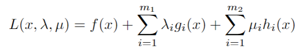
Here λ_i and μ_i are called the Lagrange Multipliers. We can then use this function to find our minimum point.

This also leads us to the following theorem — where we assume that f(x), g_i(x), and h_i(x) are differentiable (note that we don’t assume convexity yet):

We can then see what these KKT Conditions are:

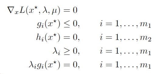
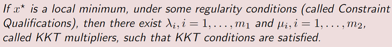
We saw before that we only assumed differentiability. However, we can then look at the following theorem:

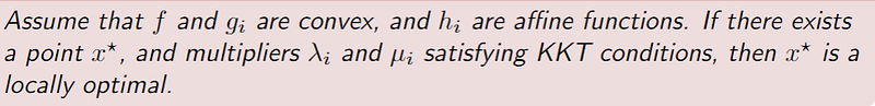
What does this say? It says that if we have a convex optimization problem, and we have found an optimal point, x*, while our multipliers satisfy the KKT conditions — then our point is guaranteed to be a local minimum.

Example of Finding the Lagrangian Function and KKT Conditions

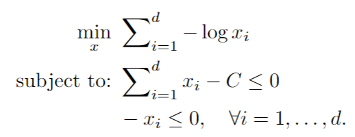
Let us now try to take a few examples, where we find the Lagrangian Function for a convex optimization problem — and the KKT conditions the problem needs to satisfy. Let us start with the problem from before, which we wrote onto the standard form:

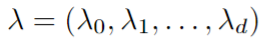
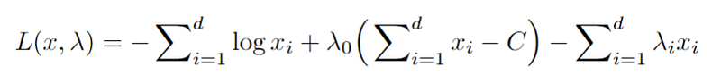
We can then try to find its Lagrangian Function. We remember that we only have g_i(x) constraints and no h_i(x) constraints. Now, if we assume that we have the following:

Then we would have the following Lagrangian Function:

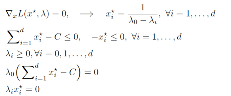
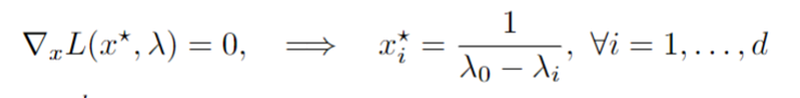
We can then also check the KKT conditions that the optimal point, x*, satisfies:

The Dual Problem

We have now seen how we can find the Lagrangian function and see which KKT conditions that the optimal point, x*, should satisfy. We will now move on to the so-called Dual Problem.

The solution to the dual problem provides a lower bound to the solution of the primal (minimization) problem. Let us try to define this Dual Problem:

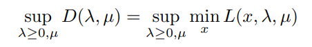
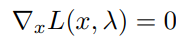
Hence, we need to first minimize our Lagrange function — which is simply done by finding:

Afterward, we need to maximize. Let us take an illustrative example.

Example of the Dual Problem

We remember our Lagrangian function:

We remember that we have found:

which then gives the following function:

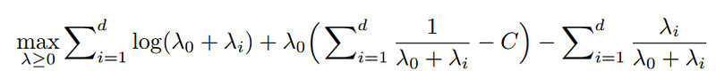
Which we would need to maximize like so:

Conclusion

We have now understood what is meant by a convex optimization problem — which we can write into the standard form. Afterward, we can solve it by either using the Lagrangian Function or using the Dual Function.

References

• Igel, C. (2021). Support Vector Machines — Basic Concepts. In Machine Learning: Kernel-based Methods Lecture Notes (Version 0.4.3). Department of Computer Science University of Copenhagen.
• Ben-David, S. Shalev-Shwartz, S. Convex Learning Problems. Understanding Machine Learning: From Theory to Algorithms. Cambridge University Press.