An Introduction to Convex Learning Problems

In this article, we will talk about Convex Learning Problems. The reason is that convex learning is an important family of learning problems since most of what we can learn efficiently falls into it this category. Therefore, in this article, we will define what is meant by a convex learning problem. To do so, we will need to just define what is meant by ‘convexity’. Besides that, we will also define concepts such as ‘Lipschitzness’ and ‘smoothness’ since they will also be needed when we define convex learning problems.

Defining Convexity

Now, let us first give a quick definition of what is meant when we talk about a convex learning problem:

A convex learning problem is a problem whose hypothesis class is a convex set, and whose loss function is a convex function.

Then we know that. However, let us first define what is even meant by something being ‘convex’, especially hypotheses classes and functions. Let us start by considering when a hypothesis class is convex. If you do not feel like you know what exactly is meant by a hypothesis class, then you can read the following article where I talk about them: Is Learning Possible? However, in a few short words — a hypothesis class is the set of possible classification functions you’re considering. For example, if you are using the Decision Tree Algorithm, then your hypothesis class is the set of all possible decision trees.

So, what does it mean when a hypothesis class is convex? As stated, it would mean that our set is convex — and the definition is given below:

A set, C, in a vector space is convex if for any two vectors u, v in C, the line segment between u and v is contained in our set, C.

Let us try to see an example of a convex and non-convex set to understand how we can check. An example can be seen below:

We can see for the non-convex set that we have found two points, u and v, such that the line between the two points is not contained in the set. Hence, it cannot be said to be convex. However, with our convex set — we can clearly see that no matter where we place our two points in our circular set, the line will always be contained inside it. Hence, it is said to be convex.

We have now seen how we can check whether a set is convex or not. Let us then move on to checking for functions. We only consider functions with a single variable, not multiple. Here, we also assume that our function is differentiable — and at least twice. Let us try to look visually at a convex and a non-convex function:

Then we can define it mathematically such that we have that:

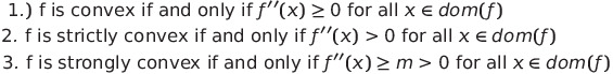
We can almost say that these conditions are in increasing order of strength. In other words, strong convexity implies strict convexity which implies convexity. Now, let us try to take a few examples.

Imagine that we have the function, which is given by:

We can then see that we have:

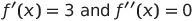
Hence, we can clearly see that it is convex — but it is neither strictly nor strongly convex.

Let us then imagine that we have the following function:

We can then see that we have:

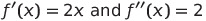
We can then clearly see that it is strictly convex since we have that 2 > 0. It is, however, also strongly convex with strong convexity constant 2.

One last thing we can say about convex functions is that there are certain rules. If f and g are convex, then f + g is convex. Furthermore, if g is strictly convex, then f + g is strictly convex, and if g is m-strongly convex, then f + g is m-strongly convex as well.

Defining Lipschitzness

We have now clearly defined convex sets and functions, and specifically how a function can also be strongly or strictly (or both) convex. Now, we will move on to talk about ‘Lipschitzness’.

Let us first give an intuitive understanding of what it is meant by ensuring Lipschitzness of a function. It simply means that we make sure that our function does not explode at some point — or in other words, a Lipschitz function cannot change too fast. Let us try to take two examples, just to get a general idea of what we want and don’t want our function to look like, if we want it to be a Lipschitz Function.

We can see that our non-Lipschitz function is becoming infinitely steep at the origin, which is exactly what we don’t want.

Now, let us try to look at it a bit more mathematically. In other words, let us get an official definition:

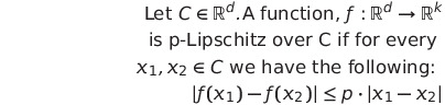
Let us try to re-arrange it such that we instead write:

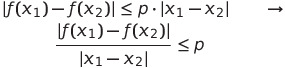
What is this equal to? Remember that the left side is the absolute value of the slope of the secant line. Hence, we’re saying that the slope of the secont line, for any two points on our graph, must be between ‘-p’ and ‘p’. We can then clearly see that this points back to our intuitive definition, a Lipschitz function cannot change too fast.

Let us try to take an illustrative example. Imagine that we want to prove that sin(x) is a 1-Lipshitz function. To do so, we will need to use The Mean Value Theorem (if you are not familiar with it, you should read this article). We remember that The Mean Value Theorem tells us that:

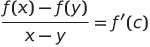
We can then use this in the case of our function, sin(x). Hence, we would write the following:

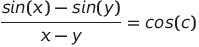
Now, we simply need to re-arrange it back to the original form in the definition of a p-Lipschitz function. We can start by taking the absolute value:

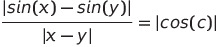
We then re-arrange such that we write:

However, we know that:

Hence, we can instead re-write to:

Here we have that p = 1, we have now proven that sin(x) is a 1-lipschitz function.

Defining Smoothness

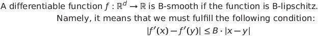
We have now defined both convexity and Lipschitzness, we will not try to define smoothness. We will need the definition of Lipschitzness to define it. Let us see the formal definition:

Let us take an illustrative example. Imagine that we have the function:

We can then find the derivative:

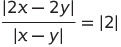
We can then check whether this is p-lipschitz. We start by again finding:

We can see that this is equal to:

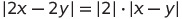
Now, we simply need to re-arrange it back to the original form in the definition of a p-Lipschitz function. We can start by taking the absolute value:

We then re-arrange such that we write:

We can then see that we have:

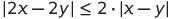
Hence, we can say that our function is 2-lipschitz, which also means that it is 2-smooth.

Convex Learning Problems

We have now defined these three concepts, and we can now go back to defining the Convex Learning Problem. We remember the definition of it:

A convex learning problem is a problem whose hypothesis class is a convex set, and whose loss function is a convex function.

Now, we will try to re-phrase it a bit. We know that we have a convex hypothesis class and we have a convex loss function. Rremember, the loss function is simply the function that computes the distance between the current output of the algorithm and the expected output. When we’re trying to learn something, i.e. choosing the right hypothesis from our set, then we want to minimze the distance between the current output of the algorithm and the expected output. In other words, we want to minimize our loss function. This leads us to the following definition:

If l(*,*) is a convex loss function and the class H is convex, then minimizing the empirical loss over H, is a convex optimization problem.

So, when we are having a Convex Learning Problem then we actually have an optimization problem, and since it’s specifically convex — then we can easily define it as a convex optimization problem. The question is of course, can we learn this problem — or, is it possible for us to guarantee that we can choose the right hypothesis? For reasons that I will not get into in this article, as it turns out — we cannot guarantee it if we only assume convexity. Instead, we will need some additional assumptions.

Making Extra Assumptions

As it turns out, we will need to consider the concepts of ‘Lipschitzness’ and ‘Smoothness’ if we want to guarantee learnability. We will therefore define ‘Convex-Lipschitz Learning Problems’ and ‘Smooth-Bounded Learning Problems’. However, before we do that, I will first formally define a learning problem (in general) since it will help us when we define these more specific ones mentioned above.

Let us then formally define a learning problem. It consists of three parameters: ‘H’, ‘Z’, and ‘l’. Here, H is our hypothesis set, ‘Z’ is the space of (input, label) example pairs and ‘l’ is our loss function. We can then define our hypothesis set, H, to be be the set of vectors ‘w’. Then our loss function can be written as l(w,z).

We can then define a ‘Convex-Lipschitz Learning Problem’. It is defined like the following:

A learning problem, (H, Z, l), is called Convex-Lipschitz-Bounded, with parameters ρ, B if the following holds:

1.) The hypothesis class H is a convex set and for all w ∈ H we have ||w||≤ B.

2.) For all z ∈ Z, the loss function, l(·, z), is a convex and ρ-Lipschitz function.

We can then also define a ‘Smooth-Bounded Learning Problem’. It is defined like the following:

A learning problem, (H, Z, l), is called Convex-Smooth-Bounded, with parameters β, B if the following holds:

1.) The hypothesis class H is a convex set and for all w ∈ H we have ||w||≤ B.

2.) For all z ∈ Z, the loss function, l(·, z), is a convex, nonnegative, and β-smooth function.

In other words, we know now that the properties of convexity, boundedness, and Lipschitzness or smoothness of the loss function are sufficient for learnability. Convexity is not enough guarantee that a problem is learnable.

Conclusion

We have now talked about concepts such as ‘convexity’, ‘Lipschitzness’, and ‘smoothness’. We also now know that convexity is not enough for us to guarantee that a learning problem to be learnable. Instead we needed the concepts of ‘Lipschitzness’ and ‘Smoothness’ to guarantee learnability.

References

• Igel, C. (2021). Support Vector Machines — Basic Concepts. In Machine Learning: Kernel-based Methods Lecture Notes (Version 0.4.3). Department of Computer Science University of Copenhagen.
• Ben-David, S. Shalev-Shwartz, S. Convex Learning Problems. Understanding Machine Learning: From Theory to Algorithms. Cambridge University Press.