A New, Better Version of the K-Nearest Neighbors Algorithm

Improve your results with KNN by using regularization

Introduction

The other day, while writing this article on the KNN algorithm, I noticed one thing: distances between observations are calculated without taking into account the importance of each feature to the overall task.

Even if you filter out the irrelevant features, the remaining ones will still have different levels of importance for predicting a certain target variable, and that is not considered when we identify the nearest neighbors.

I then tried to find implementations of KNN or articles that would do that, but nothing came up (I found this article that seems to do something similar, but it is not very clear on how the weighting is done, nor it has any implementation). Finally, I decided to do it myself, test if it could improve results and then put it out there so that other people could improve it.

This article will then present the theory behind this method of “regularization” for KNN, Python code to implement it, results on a toy dataset and suggestions for further improvement.

KNN

Let x be a new observation for which we want to estimate the value of the target variable y. The KNN algorithm works as follows: 1. Calculate the distance between x and all the other data points for which we know the the value of y. 2. Arrange the distances in increasing order 3. Given a positive integer k, select the k-first distances from the arranged list 4. Select the k points corresponding to those distances 5. If it’s a classification task, label x with the majority class amongst the k observations. If it’s a regression task, estimate y using the average value of y for the k observations.

The distance measure used on step 1 can vary according to the task in hand and the type of data, but most common ones include Euclidean, Manhattan, Minkowski and Mahalanobis distances.

Intuitively, this means that when we want to predict a value for a new observation, we find similar observations for which we have that information, and base our prediction on those known values.

Regularized version

On the KNN algorithm, regularization can be done during step 1, when calculating the distance measure between x and the other points. In order to take into account the relationship between each variable and the target, we have a few alternatives. In this article, we’ll use the absolute value of the Pearson correlation coefficient as a weight for each feature, adjusted by a regularization parameter:

where j represents the rank of the feature in question, and λ represents the regularization parameter. The greater the regularization parameter is, the more it penalizes features that are not correlated to the target variable, and the less they will weight in the distance calculation.

That has the advantage of being non-negative and easily interpretable. On the downside, it will not properly take into account non-linear relationships.

A weight vector w can then be formed from the weights of each feature, and then be applied to the Minkowski distance:

Or to the Mahalanobis distance:

Implementation

The following steps were followed in order to evaluate the regularized KNN predictive power: 1. For each distance metric (Manhattan, Euclidean and Minkowsky), the local optimal value for k was calculated within a certain arbitrary search space, using the non-regularized version of KNN and optimizing for the MSE (Mean Squared Error) 2. That same k was applied to the regularized version, using different values of λ 3. The MSE scores obtained by both algorithms were then compared to identify the optimal solution

Results

In order to test its predictive power, the regularized version has been tested on the diabetes dataset included on sklearn.

The dataset contains information on health indicators and diabetes, with 442 instances and 10 attributes, one of which being the target variable for our regression task: a quantitative measure of disease progression one year after baseline. All other variables are numeric or binary, and include information such as age, BMI and sugar blood levels.

Regularizing the KNN algorithm yielded better results for all three distance metrics, and the best overall MSE (3314) was obtained with the regularized version of the Mahalanobis distance:

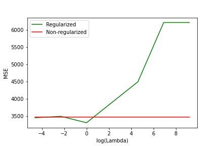
As we can see, results can vary significantly depending on the value used for λ (the regularization parameter) but it still shows that regularizing the KNN algorithm can lead to improvements.

Conclusions and further research

A potential area of further improvement would be to replace the Pearson’s correlation coefficient by another metric that takes into account non-linear relationships. If you have any suggestions, please comment them below!

The full code used for the tests and a more detailed paper on this topic can be found here.

If you liked this article, you will probably like these ones too:

Feel free to reach out to me on LinkedIn if you would like to discuss further, it would be a pleasure (honestly).