Support Vector Machine: Theory and Practice

Understand SVM, one of the most robust ML algorithms out there

Introduction

Support Vector Machine (SVM) can be used for regression and classification tasks (although it’s more commonly used for classification), and its goal is to find the hyperplane that best distinguishes the data points (we’ll get back to that later). It is a simple but powerful algorithm, that every data scientist should know and, in this article, we’ll go through the ins and outs of its classification version.

Intuition

To get a first intuition of how SVM works, imagine a guy entering a party (note for data scientists: a party is a social event where people gather to drink, chat and dance). This party is filled with two big groups of people talking, and the guy doesn’t feel like talking to either of them right now, he just wants to cross the venue to get to the bar and have his first beer. To get to the other side, he doesn’t want to cross into the middle of any of those groups, because it could be awkward to walk through the middle of their conversation. He also doesn’t want to get too close to any of these groups, because someone might spot him and start chatting, and that would distract him from getting his first beer. So he goes, trying to walk in between the groups, keeping the largest distance he can from all of them.

That is roughly the way SVM works, by creating a “line” that goes through different classes, avoiding splitting observations from the same class, while keeping the largest distance possible from those classes.

In order to understand SVM, we have to go through a couple of its fundamental concepts: hyperplanes and their margins.

Hyperplanes

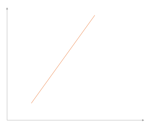
No, hyperplanes are not super-powerful airplanes. A hyperplane is a “subspace whose dimension is one less than that of its ambient space”. So, for instance, in a 2-D ambient space, that would be a line:

In a 3-D ambient space, a hyperplane is a 2-D subspace:

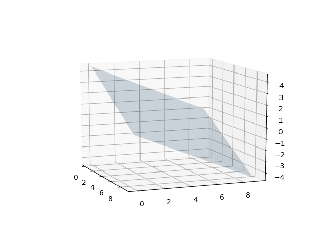
Easy, right? You can have it for higher dimensions too, but then it becomes more complicated to visualise.

Margins

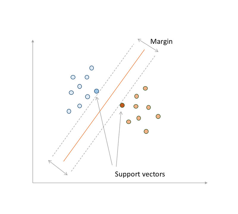
Now, imagine that there are some points in your space and they are more or less separated in 2 groups. The margin would be the minimal distance between the closest points in each group and your hyperplan. Those closest points to each group are called support vectors, by the way, and they are important because they are the hardest ones to classify, since they are the points, within their groups, that are the closest to the other group. In 2-D, the margin would be something like that:

SVM

Now that you know what hyperplans and margins are, you can probably guess where this is going. An SVM learning algorithm will try to find the hyperplane that maximises that margin. That way, we’ll have a reasonable boundary splitting the classes, and everything that falls on one side of the hyperplane will be assigned to one class, while everything that falls on the other side will be assigned to the other class. The hyperplan will work as a decision boundary.

The basic case

How does that learning algorithm works? Well, let’s call the input feature vector x. We can write the equation for the hyperplan using two parameters: a vector a that has the same number of dimensions than x, and b, a real number. The equation would look like this: ax — b = 0 (think of our 2-D example, where our hyperplan is a straight line). Now let’s say our variable of interest, that represents the classes, is called y, and equals to -1 or 1, depending on the class. In our equation, that would mean: y = sign(ax — b), where sign returns -1 if the equation within it is negative, and 1 if its positive.

What SVM does is try to find the best values for a and b, which we’ll call a* and b*. The model f(x) will then be defined as f(x) = sign(a*x — b*). Then, to predict a class, all we would have to do is plug in our values of x to that function and get an answer. Great! But how exactly do we find those optimal a and b? Well, as the name says, it’s an optimisation problem.

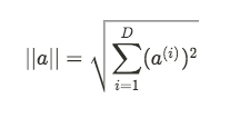
More specifically, we want find the a and b parameters that maximise the margin, which is given by the distance between the two hyperplanes. Those hyperplanes are formed by the equations ax — b = 1 and ax — b= -1 and the distance between them is given by 2/||a||, where ||a|| is the Euclidean norm of a:

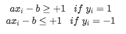
This means that, if we minimise ||a||, we maximise our margin. But we also have 2 constraints, that exist so we make sure that examples from the same class fall on the same side of the hyperplan:

Usually, the method used for this optimisation problem is the method of Lagrange Multipliers.

Non-linearity

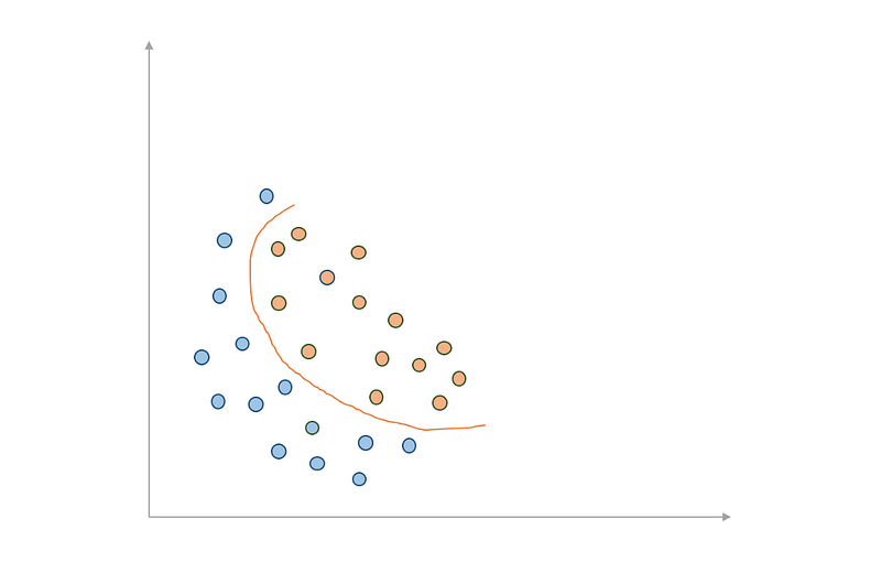
Ok, it’s all fun and games so far, but real-life data will hardly ever look like this. First of all, let’s deal with the linearity assumption. It might happen that our data is just not linearly separable, in which cases you want your boundary to take that into account:

What do we in these cases? Well, we can turn to non-linear SVMs, which map data to a higher dimensional space in order to find a way to separate it linearly, by using what is called the kernel trick.

Kernels are similarity functions between an observation x and a landmark vector l. There are many possible Kernels, and you can choose which one you want depending on how your data looks like (including a linear Kernel). In our 2-D space, we could generate 3 landmarks and measure the similarity between each observation and each landmark, and transform that into a new feature vector. Now, instead of having 2 features, each observation has 3 (its similarity with each of the landmarks). In that new feature space, we might be able then to find a linear boundary.

Too much noise

In some cases, it might be impossible to perfectly separate data, even with non-linear SVMs. For those cases, there are SVM versions that don’t impose the constraint that every observation is correctly classified but, instead, calculate a loss function, penalising such cases (and then work to minimise that cost). This is, of course, the most frequent case.

That loss function is then combined with the margin to give us a cost function, that we’ll then try to minimise:

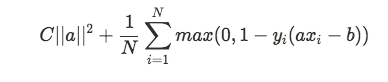
What we are doing here is multiplying the margin by a parameter C that will essentially decide how much weight we want to attribute to the margin as opposed to the loss generated by a misclassification. That loss is either 0, if our classification is correct, or a proportion of the distance between the observation and the decision boundary, if our classification is incorrect (actually, the average of that across every observation, given that N represents the number of observations).

That parameter C gives us some freedom to decide how much we want to penalise bad predictions in order to have a better margin for our decision boundary (that is, how much we want to risk overfitting in order to have a “better” classifier). The higher C is, the more we bend our hyperplan to fit all the observations and the more we risk overfitting.

How to use SVM in practice

Let’s imagine a classification task where you have 2 classes and 2 explanatory dimensions and try to use SVM to solve it in Python (I’m picking this simple 2-D case because it’s a lot easier to visualise, but the same technique will apply for higher dimensions). The full code is available here.

IN:
import numpy as np
import matplotlib.pyplot as plt
from sklearn import svm
from sklearn.datasets.samples_generator import make_blobs

First, we just import the libraries we need (the most important import here is svm from sklearn).

IN:
# Generate data
X, y = make_blobs(n_samples=100, centers=2,
 random_state=123, cluster_std=3)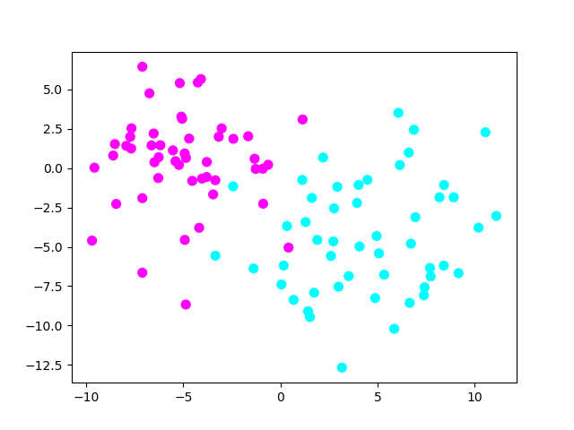

We have then generated artificial data. As we can see, our data is not linearly separable (nor completely separated, as there is some noise).

IN:
# Fit model
clf = svm.SVC(kernel=’linear’, C=0.1)
clf.fit(X, y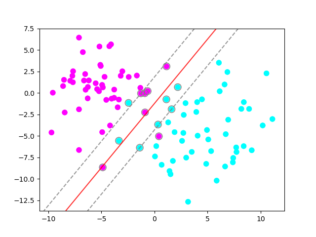

Here, what we did was fit a Support Vector Classifier (hence the SVC), using a linear kernel and a C of 0.1. If this was a regression task, we would be using SVR instead of SVC. Now, let’s try using a non-linear kernel to see how it will fit our data:

IN:
# Fit model 2
clf2 = svm.SVC(kernel='poly', C=0.1, degree=3)
clf2.fit(X, y)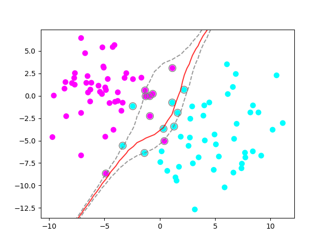

So, this is a polynomial kernel of degree 3. We can see how it tries harder to fit to the data we have, which might result in overfitting. Let’s now look at another possible kernel, called Radial Basis Function (RBF).

IN:
# Fit model 3
clf3 = svm.SVC(kernel=’rbf’, C=0.1)
clf3.fit(X, y)
plot_classifier(X, y, clf3)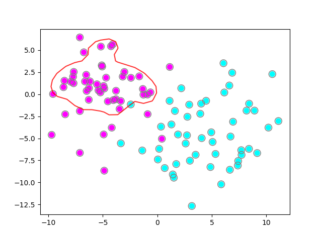

It looks like our model is under-fitting, misclassifying many of the pink exemples. Let’s try increasing the C parameter to see its effect:

IN:
# Fit model 4
clf4 = svm.SVC(kernel=’rbf’, C=1)
clf4.fit(X, y)
plot_classifier(X, y, clf4)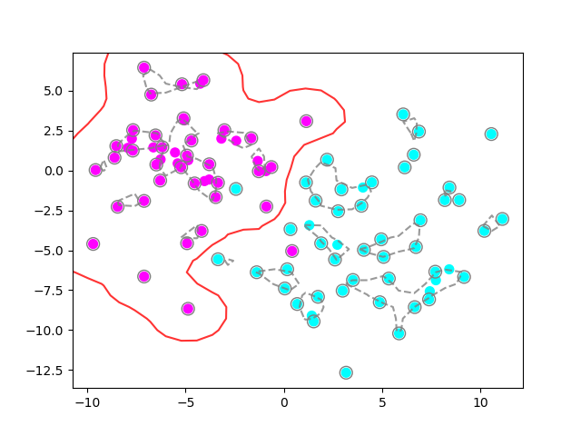

It looks a lot more reasonable now, right? Still, if we have new pink observations that are too far to the left, they will be misclassified as blue, since our boundary is closed around the pink blob, which could also indicate overfitting.

If you want to read more about the different kernels and how to use it, check out the scikit-learn documentation here.

Extra tips

• SVM works well with high dimensional data (it can still work well even when you have more dimensions than observations). However, when that is the case, choosing the right Kernel function and regularisation term (the C paramter) is crucial to avoid over-fitting.
• If memory is an issue, know that SVM is quite memory-efficient, since it uses only the support vectors in the decision function.
• If needed, in scikit-learn you can use the decision_function method of SVC, with the constructor option probability set to True, to get probability estimates for each observation (you can read more about it here).

Conclusion

Congratulations, you have now added SVM to your arsenal as a data scientist. SVM is a powerful and easy-to-understand algorithm and hopefully, by now you have an intuitive grasp of how it works, including the mathematics behind it. For extra knowledge, go check the scikit-learn documentation to see how you can tweak all its different parameters.

If you like learning how ML algorithms work and how to apply them, you might also like this article on XGBoost:

Feel free to reach out to me on LinkedIn if you would like to discuss further, it would be a pleasure (honestly).