Maintain a Companion Plant Knowledge Graph in Google Sheets and Neo4j

Store data in tables and gain insights from graphs

Even though there was enough food for 10 billion people, 10% of the world population still regularly goes to bed hungry. Climate change, COVID-19, and the war in Ukraine have exacerbated the food crisis. While feeding the world population (8 billion in 2022) has already been hard enough, producing and distributing enough food for the future population (9.8 billion in 2050) will be even more challenging, especially when the losses of topsoil, agricultural knowledge, and soil biodiversity keep acting against us.

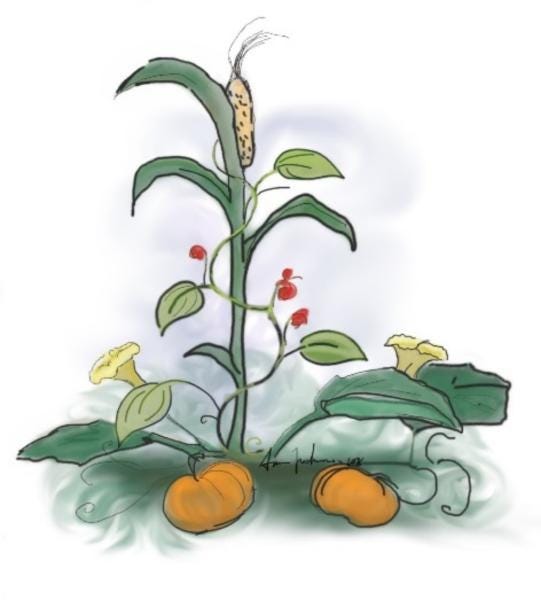
In the face of a large-scale food crisis and climate change, we need to reform our current unsustainable agriculture. Among the several alternatives, such as hydroponics and aquaponics, the good old companion planting is really worth our attention. It is the farming practice of growing diverse plants in proximity that support each other either by nutrient provision, beneficial insect attraction, or pest suppression. In comparison with monocultures, companion planting can be more productive and more eco-friendly. One well-known example is the Three Sisters: winter squash, corn, and beans (title figure). Beans fix nitrogen with their symbiotic bacteria. Squash protects the soil from the elements with its broad leaves and repels pests with its hairs. And corn is a natural trellis for the beans to climb. Together, they can protect the soil from erosion and increase productivity.

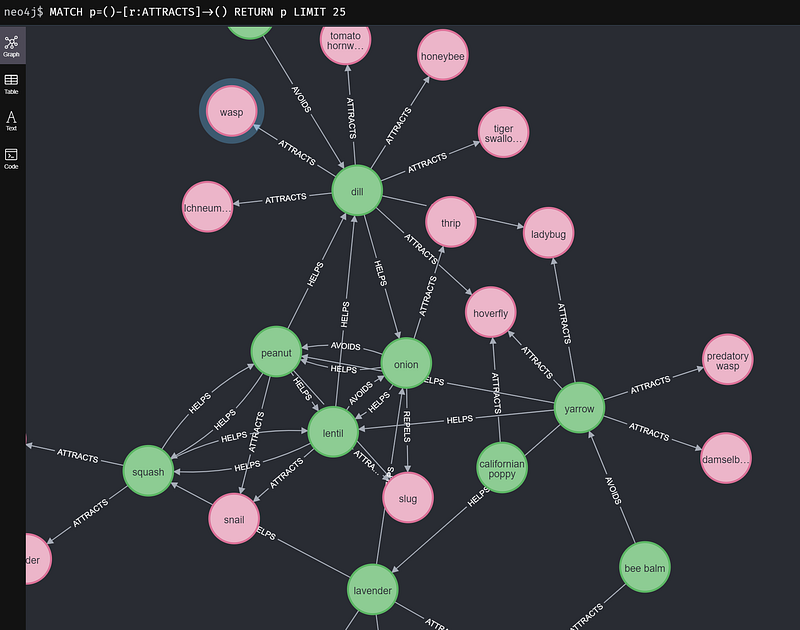
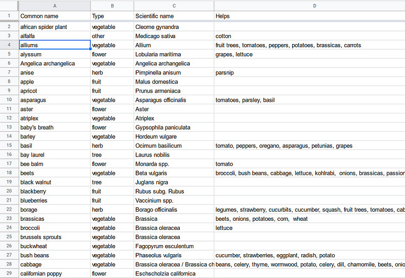
Humans have practiced companion planting over millennia and accumulated extensive knowledge about the subject. This knowledge is codified into tables, such as this one on Wikipedia. Tables are easy to modify and maintain with tools such as Google Sheets. But for relation-rich data such as the companion plant data, a table is not my first choice for visual analysis. In contrast, a network graph (Figure 1) can display the intricate interconnections of plants easily. We can also perform graph queries and graph-based algorithms to gain new insights into the data.

But data editing in a graph database like Neo4j is not as simple as in a table. Although the graph app Neo4j Commander brings data editing into the Neo4j platform, its user experience is still a far cry from what we can get from Google Sheets. Can we have both easy data editing and easy graphing with just one single source of truth?

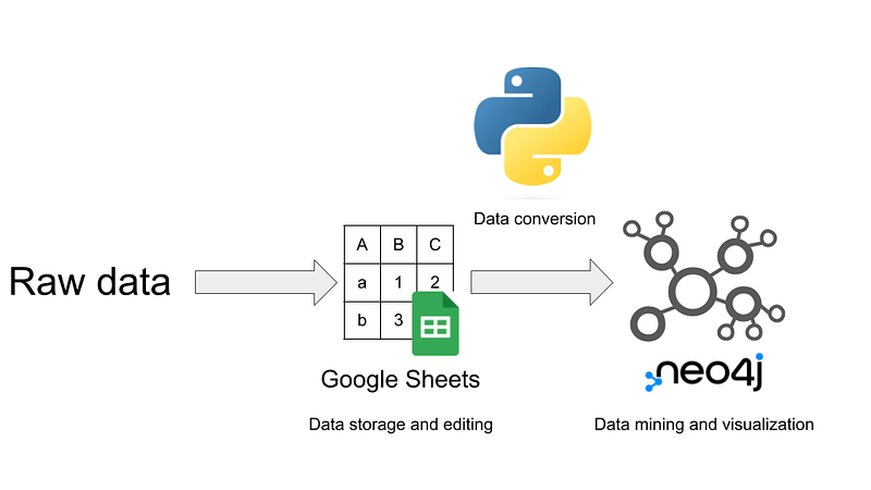
In this article, I want to show you my solution. I store the companion plant data from Wikipedia in Google Sheets. It is my only source of truth. I then use Neo4j Desktop to create a local knowledge graph. A Python Jupyter notebook serves as a bridge. The notebook downloads and formats the data from Google Sheets. Then it drops the old data and imports the new one in Neo4j (Figure 1). And then we are going to do some data mining on the knowledge graph in both Cypher and Python. For example, I am going to use the Degree Centrality algorithm in Neo4j’s Graph Data Science (GDS) library to calculate the largest set of mutually supportive plants that we can grow around the potatoes.

The code for this article is hosted on my GitHub repository here.

The data in this project comes from Wikipedia and is under the Creative Commons Attribution Share-Alike license. The Google Sheet is here.

0. Preparation

First, create a Neo4j project in your Neo4j Desktop called “companion plants”. Open its import folder (“…” ➡️ “Open folder” ➡️ “Import”). Copy the seemingly random database string (dbms-xxxxxx) and set it as the value of neo4j_project_id in config.yaml. Also, fill out the other details in config.yaml.

In addition, you need to enable the GDS library in the Plugins tab.

1. Load the companion plant dataset into Google Sheets

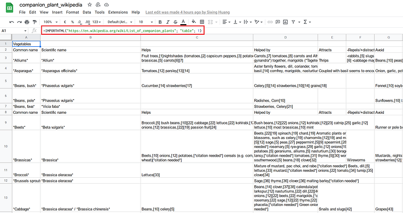
My table is based on the List of companion plants on Wikipedia. The data were split into five tables: vegetables, fruit, herbs, flowers, and others. I then used the IMPORTHTML function to fetch the data into five Google Sheets and merged them into a master table.

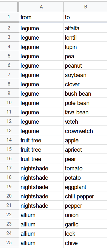
Afterward, I manually curated the data. I first corrected several typos, cleared some ambiguous terms like “almost everything”, added many data entries, and normalized the synonyms (Figure 3 left). Finally, I constructed a sheet for the taxonomy (Figure 3 right).

For simplicity’s sake, I made the Google Sheets generally accessible so that the pandas library could load the data easily later in my script. And because the data are in the public domain, it is OK for this project. But if your project data are confidential, you’d better set a more restrictive access policy in Google Sheets and use the gsheets library in your Python script.

2. The Python bridge

The middleware consists of three files: a Jupyter notebook, a config.yaml, and a text file containing all the Neo4j commands. Config.yaml contains the local Neo4j credentials and other user data. The Python Jupyter notebook connects Google Sheets with my Neo4j database.

Data from Google Sheets can be read directly with the read_csv function in pandas (Listing 1).

Then the script iterates the cells in the table and split the comma-delimited contents. They are mostly plant and animal names. The script singularizes the plural forms, resolves the synonyms, and concretizes the umbrella taxa (“legume” into “bush bean”, “alfalfa” and so on)(Listing 2). It also stores the nodes and relations in variables such as nodes_plant and plant_plant_help.

Afterward, the script writes these variables into TSV files. For example, the code below creates the file for the plant nodes.

The script then connects to the local Neo4j instance and clears all constraints and old contents.

Then it copies all the newly generated TSV files into my project’s import folder.

Finally, the script carries out the import commands in the neo4j_command.txt file. These commands import the TSV files into the knowledge graph and create the corresponding constraints.

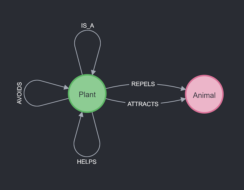
And the knowledge graph has the following simple schema. It represents the supportive and antagonistic relations among various plants and animals.

3. The companion plant knowledge graph

Once the data are loaded, we can start exploring the knowledge graph. There are 162 plant nodes, 71 animal nodes, and 2,182 relations in the graph. Among the relations, we observe 1,455 HELPS and 404 AVOIDS relations.

3.1 Which plants are good companions for tomatoes?

If we want to grow tomatoes, let’s find out which plants are good companions.

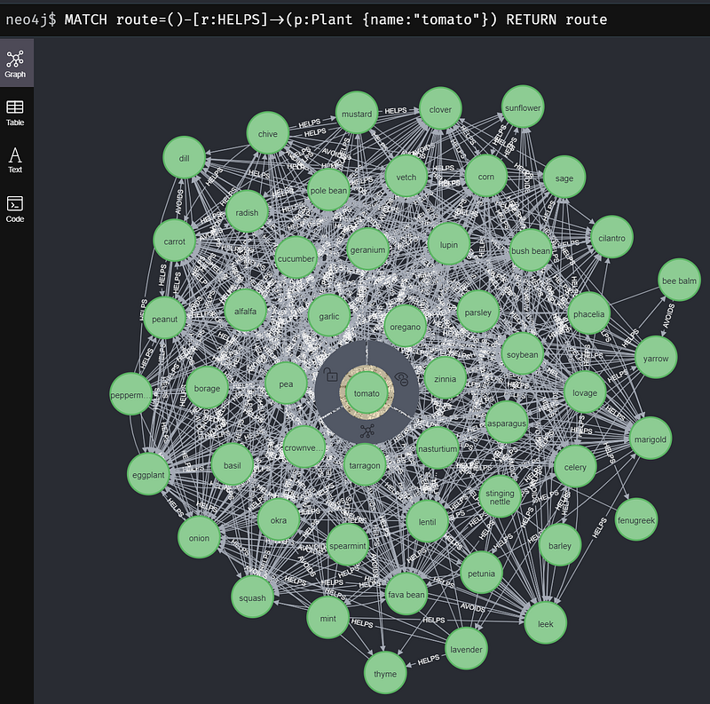
It turns out that many plants can help us to grow tomatoes. For example, basil, borage, garlic, and marigold can all repel pests, while chive, mint, and parsley can make tomatoes healthier. But we should avoid cabbage, fennel, and walnut tree.

3.2 The most avoided plants

As the example above shows, there are antagonistic combinations that we’d better avoid growing together. For example, walnut synthesizes an allelopathic compound called juglone that can inhibit the growth of tomatoes. Here, let’s see which plants are the most avoided in the dataset.

According to Wikipedia, the number one should have been flax. However, that data entry has been flagged as “citation needed” and I could not verify that information anywhere else. On the contrary, flax can promote tomatoes and potatoes because it can repel Colorado potato beetles. To be on the safe side, I cleared its AVOIDS relations. And then fennel becomes the number one. The root of fennel secrets substances that inhibit and even kill many garden plants. In fact, dill is the only thing that can grow next to fennel. Other than that, plant it by itself [1].

3.3 Calculate the largest AVOIDS-free, supportive plant network for the potatoes

Let’s assume that we want to plant potatoes in a large field. And we want to plant the most biodiverse set of plants there. There is one restriction though, no “AVOIDS” relation is allowed in the community. In other words, there should not be any antagonistic plant pair in the set. Notice that there can be multiple such optimal lists.

I googled it but could not find any solution. So I developed two algorithms myself in Python. Both algorithms begin with the list of plants that can promote potato growth.

This initial list contains alfalfa, brassica, garlic, lovage, and so on.

For each plant, I count how many AVOIDS relations it has against the others (Line 12–19 in Listing 11).

In the first round, garlic does not grow well with the other thirteen plants on this list. It is also the plant with the most AVOIDS relation. So I remove garlic from the supportive plant list (Line 24–29 in Listing 11). The algorithm then repeats this process (Line 8–29 in Listing 11) until no more AVOIDS relation can be found. If there are more than one plants with the same amount of AVOIDS, the code removes one of them randomly (Line 25–27 in Listing 11).

In one of my runs, this algorithm successively removes garlic, leek, chive, onion, and so on. The final list contains the following 22 plants: alfalfa, basil, cabbage, carrot, clover, corn, crownvetch, dead nettle, flax, horseradish, lentil, lovage, lupin, marigold, mint, pea, peanut, pole bean, soybean, tarragon, vetch, and yarrow.

The second algorithm uses Degree Centrality from GDS to decide which plant to remove in each iteration. The Degree Centrality algorithm is used to find popular nodes within a graph. In our case, I use it to find the most avoided plants. The algorithm measures the number of incoming or outgoing (or both) relationships from each node and stores the metric in the “score” column in a pandas dataframe. Its implementation differs from the first one in the “while” loop.

During each iteration, this algorithm first projects the supportive plants and their AVOIDS relations into a graph object (Line 14–17 in Listing 12). Then it calculates the degree centrality score for each plant (Line 19 in Listing 12), fetches the most “popular” one (Line 20–26 in Listing 12), and removes it from the supportive plant list. When there are multiple plants with the same degree centrality score, the code removes one of them randomly. The algorithm repeats itself until all degree centrality scores are 0 (Line 34–35 in Listing 12).

This algorithm finds a new set of 22 plants each time you run it. But some of the plants, such as yarrow and dead nettle, will always be in the set because they do not have any AVOIDS relation in the subgraph. Both algorithms are valid. You can verify the results by showing that there is no AVOIDS relation between any two plants.

But the Degree Centrality method ran in 0.4 seconds whereas my first algorithm finished in 2.6 seconds.

Conclusion

This article has shown you how I encoded the intricate plant relations into a knowledge graph with Google Sheets and Neo4j. The commensal, symbiotic, and allelopathic relations among plants are complex and awe-inspiring. We can make good use of this knowledge in companion planting. Through companion planting, we will not only reduce the use of fertilizer and pesticide, but also make the plants more resilient and tastier. Finally, it can also help us reduce the amount of irrigation. This latter point is especially pertinent in the face of the current unprecedented worldwide drought.

The table-graph combination has the best of both worlds. In essence, the workflow in this article marries a relational database with a graph database. We can edit data easily in tables and analyze them easily in graphs. I used Google Sheets in this project. But for other large projects, we can use PostgreSQL or even Snowflake or BigQuery. Once the data is loaded on a graph platform like Neo4j, we can use graph queries and algorithms to examine the data and gain interesting results with either Cypher or Python. You can read this and this by Tomaz Bratanic to learn more about using GDS in Python. The Python bridge also allows us to control which subset of the data flows to the graph. This is especially valuable when your complete dataset is too large to fit into a small Neo4j instance, you can select and import the relevant subset only. Or when we are working in a team, we can slice and then deliver the data according to the request or access level of each team member. In fact, the drug company AstraZeneca has constructed a similar data flow in their internal knowledge graph application.

By encoding the companion plant table into a knowledge graph, I have made this valuable agricultural know-how searchable and extendable for all. But there is room for improvement, too. Can you suggest a better algorithm to calculate the largest AVOIDS-free, supportive plant set for the potatoes? And I encourage you to validate the information in this knowledge graph or even make your own version.