
Z-scores in Investing and Finance: Are You Using Them Right?

When risk managers or quant professionals need to compare different metric types or normalize data, z-scores are their go-to measure. In theory, Z-scores are powerful and easy to understand. In practical use, however, they have two strong limitations that can affect their interpretation:
- A high sensitivity to the distribution of underlying data
- Their interpretations relative to each other
When using a z-score for finance or investing, these limitations have real-world consequences.
Deep Dive: What Is a Z-score?
A z-score is defined as ‘a numerical measurement that describes a value’s relationship to the mean of a group of values’. Essentially, it is a measure of how far a data point deviates from the mean. Z-scores are often used to normalize raw data because they show the standard deviation below or above the average value.
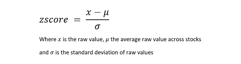
To calculate a z-score, you need three numbers: the mean (the average raw value), the value of your data point (the raw value), the standard deviation of all data points within the dataset (standard deviation of raw values). This calculation is simple to understand and explain, which is why z-scores are so popular in finance and investing.
Z-score Interpretation
So, what is a good z-score? Well, knowing the definition of a z-score won’t get you anywhere unless you also understand interpretation. There are several ways to interpret results, and this is where the limitations of z-scores come into play.
First, let’s look at a dataset. Below is a dataset containing the height of a population. It’s in the shape of a bell curve, which I’ll talk about shortly. Let’s say you pull someone’s individual height from this data: an individual that is 180cm tall (5’10”). Looking only at that number provides no indication of how it relates to the data set. Is the person tall or close to average height?
When converted to a z-score, you get the number 1.17, which means the individual is in the top 12% of the population with a height of 180cm, assuming your distribution follows a normal law.
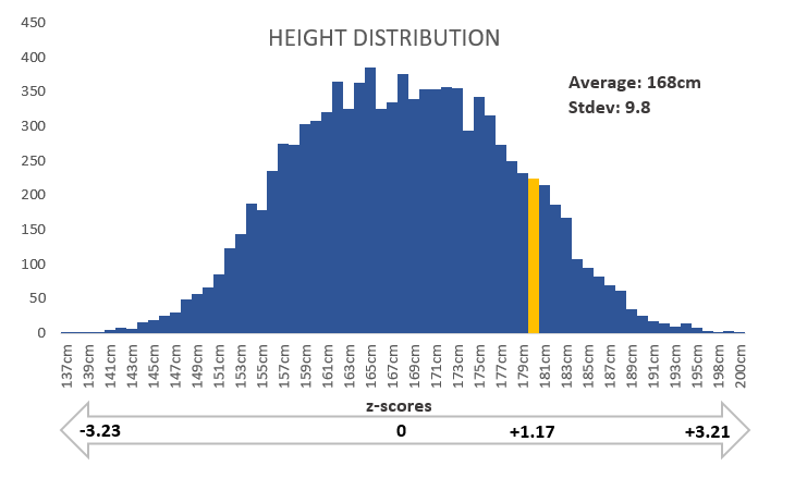
Investors and those in finance often look at z-scores with the bell curve in mind. A bell curve, or normal distribution, gets its name from its shape, which resembles a bell. The chief characteristic of a bell curve is its ability to incorporate 68% of its data within -1/+1 standard deviation from the mean, 95% of data within 2 standard deviations, and 99.7% of data for 3 standard deviations. A bell curve offers an easy way to analyze a z-score. Hence, why it’s so popular.
For example, a score greater than 3, meaning 3 standard deviations from the mean, is significant because there’s only 0.15% of data with greater z-scores. In comparison, a z-score of -2 has only 2.5% of data below that threshold.
This brings us to the first limitation of z-scores.
Z-scores Are Highly Sensitive to the Distribution of Underlying Data
In the real world, datasets don’t always follow the bell curve. Actually, very few datasets offer normal distribution, one of the biggest drawbacks of z-scores. If you don’t know the distribution of your underlying data, it’s hard to know how to interpret a z-score. For example, is it still correct to assume that the previous 0.15% of data have a z-score greater than 3?
To understand my point, let’s look at the market cap of stocks. The vast majority of stocks are below a billion dollar market cap, and few of them go above $100 billion (only some giants like Apple, Microsoft or Amazon). Because of this, market cap distribution is skewed toward smaller market cap stocks.
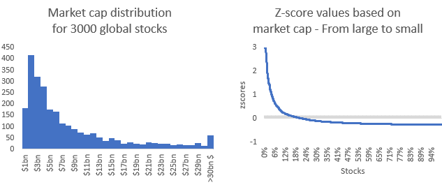
When dealing with z-scores, this distribution is less than ideal. From the chart above, you can see that most of the z-scores are below 0. A stock with a market cap of $11.8bn (the minimum requirement to be part of the S&P500 large cap index) has a z-score close to 0. Yet, this stock is considered a large market cap stock (or large cap) in finance. If the underlying dataset was normally distributed, the z-score would be close to +1, revealing that it is actually a small market cap stock.
Even worse, the smallest market caps have a z-score around -0.5. If you interpret this z-score using the bell curve, it would be considered an average market cap, despite the reality of it being among the smallest market caps.
Clearly, z-scores have the potential to offer inaccurate results if someone isn’t aware of this limitation. There is a fix, though.
Quick Fix for the Distribution of Underlying Data: Compute the Z-score of Z-scores
Thankfully, there is a way to convert z-scores so they can be interpreted as if their underlying data was normally distributed. You simply need to compute the z-score of z-scores until you get a mean of 0 and a standard deviation of 1.
To see this in practice and learn how to code it, check out my article:
Z-score Interpretation Gets Confusing in Relation to Other Z-Scores
This limitation comes up mainly when interpreting factor investing and factor models. In factor investing, professionals often use z-scores to assess the exposure of a stock with a style factor: Value, Momentum, Low Risk, Quality, or Size. However, a higher z-score does not always mean a higher exposure to a factor. In an ideal world, the greater the z-score, the more sensitive a stock would be to the underlying factor. In theory, a z-score of 2.5 would be better than a z-score of 2.4. But in the real world, this doesn’t hold up. It all depends on the behavior of investors.
When building a factor strategy, investors rank stocks based on their value for the given factor. After that, they go long on the top stocks and eventually go short on the bottom ones. The problem, though, is nothing is done to differentiate between stocks within the long or short basket. Stocks within each basket are assumed to be equally exposed to the given factor. Most style ETFs and factor indices are built this way.
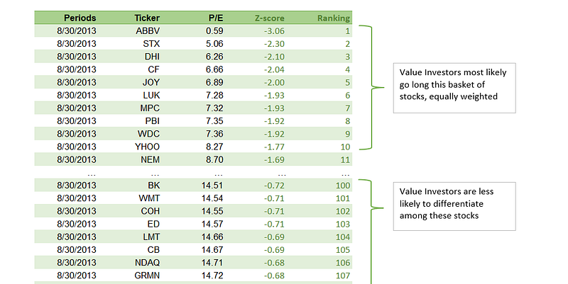
For example, if a group of investors all follow a Value strategy and buy the same basket of stocks, they will push the price up for all purchased stocks. Any distinction among them is overlooked. When translated into z-scores, this means that investors will see a difference between a stock with a z-score of 1 versus a stock with a z-score of 2, but they are less likely to notice a difference between two stocks with respective z-scores of 2 and 2.1.
Conclusion
As I’ve demonstrated, z-scores are a powerful way to normalize data because they are easy to understand and easy to explain. Yet, z-scores have major limitations that many don’t think about. First, if you don’t know the distribution of your underlying data, it’s hard to know how to interpret a z-score. Second, in factor investing, investors usually buy a basket of stocks based on a given factor, but they don’t differentiate among the stocks within the same basket. Two stocks with close z-scores won’t behave differently, even though they may have apparent differences when interpreted separately.
Z-scores are wonderful, often magical measures for finance and investing, but proceed with caution. Make sure you understand the distribution of your data and the context in which your z-scores will be used.
To learn more about the use of z-scores for factor models, check out my article about equity factor models.


