Your Random Forest Model is Never the Best Random Forest Model You Can Build
The coolest trick to improve random forest models.
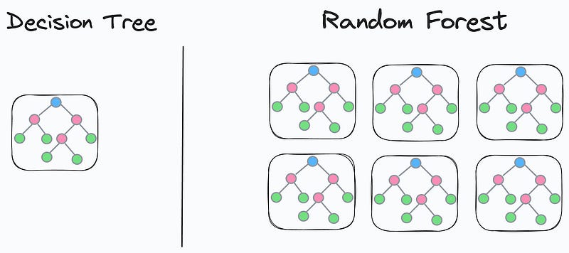
Random forest is a pretty powerful and robust model, which is a combination of many different decision trees.
But the biggest problem is that whenever we use random forest, we always create much more base decision trees than required.
Of course, this can be tuned as a hyperparameter, but it requires training many different random forest models, which takes time.
Today, I will share one of the most incredible tricks I formulated recently to:
- Increase the accuracy of a random forest model:
- Decrease its size.
- Drastically increase its prediction run-time.
And all this without having to ever retrain the model.
Are you ready?
Let’s begin!
Logic
We know that a random forest model is an ensemble of many different decision trees:
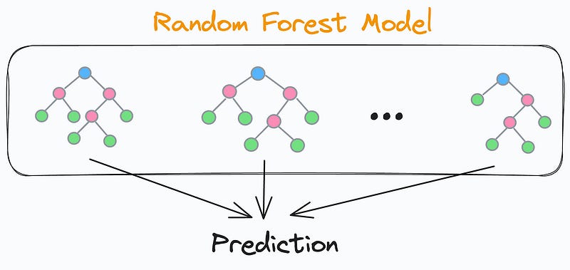
The final prediction is generated by aggregating the predictions from each individual and independent decision tree.
As each decision tree in a random forest is independent, this means that each decision tree will have some test accuracy, right?
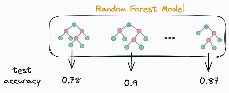
This also means that there will be some underperforming and some well-performing decision trees. Agreed?
So what if we do the following:
- We find the validation accuracy of every decision tree.
- We sort the accuracies in decreasing order.
- We keep only the “k” top-performing decision trees and remove the rest.
Once done, we’ll be only left with the best-performing decision trees in our random forest, as evaluated on the test set.
Cool, isn’t it?
Now, how to decide “k”?
It’s simple.
We can create a cumulative accuracy plot.
It will be a line plot depicting the accuracy of the random forest:
- Considering only the top two decision trees.
- Considering only the top three decision trees.
- Considering only the top four decision trees.
- And so on.
It is expected that the accuracy will first increase with the number of decision trees and then decrease.
Looking at this plot, we can find the most optimal “k”.
Implementation
Let’s look at its implementation.
First, we create a classification dataset:
First, we train our random forest as we usually would:
Next, we must compute the accuracy of each decision tree model.
In sklearn, individual trees can be accessed with model.estimators_ attribute.
Thus, we iterate over all trees and compute their validation accuracy:
The model_accs is a NumPy array that stores tree id and its test accuracy:
Now, we must rearrange the decision tree models in the model.estimators_ list in decreasing order of test accuracies:
This list tells us that the 99th indexed model is the highest performing, followed by 59th indexed, and so on….
Now, let’s rearrange the tree models in model.estimators_ list in the order of model_ids:
Done!
Finally, we create the plot discussed earlier.
It will be a line plot depicting the accuracy of the random forest:
- By considering only the top two decision trees.
- By considering only the top three decision trees.
- By considering only the top four decision trees.
- and so on.
The code to compute cumulative accuracies is demonstrated below:
In the above code:
- We create a copy of the base model called
small_model. - In each iteration, we set small_model’s trees to the first “k” trees of the base model.
- Finally, we score the
small_modelwith just “k” trees.
Plotting the cumulative accuracy result, we get the following plot:
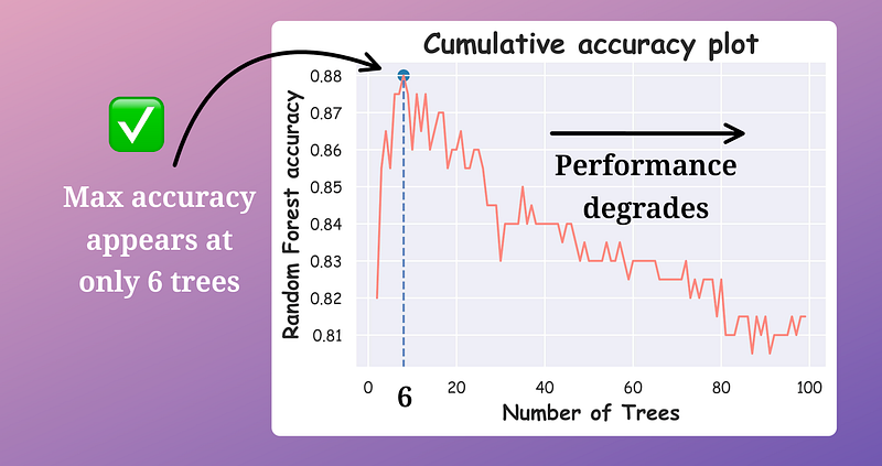
It is clear that the max test accuracy appears by only considering 6 trees, which is a sixteen-fold reduction in the number of trees.
Comparing their accuracy and run-time, we get:
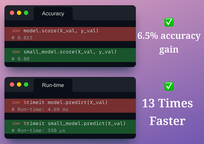
- We get a 6.5% accuracy boost.
- 13 times prediction faster run-time.
Now, tell me something:
- Did we do any retraining or hyperparameter tuning? No.
- As we reduced the number of decision trees, didn’t we improve the run time? Of course, we did.
Isn’t that cool?
Of course, we may not want to overly reduce the ensemble size because we want to ensure our RF still maintains many different types of decision trees.
The approach to select the best “k” can be quite subjective and it does not necessarily have to rely solely on the validation accuracy.
In fact, we can consider the test set to see how the reduced model is performing, as shown below:
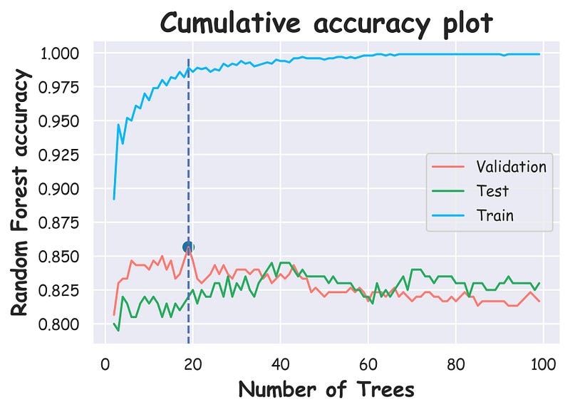
In the above plot:
- The red depicts the validation accuracy obtained after selecting the first “k” decision trees.
- The blue line depicts the corresponding train accuracy.
- The green line depicts the test accuracy..
As I mentioned earlier, the selection of decision trees does not necessarily have to be on the validation set as it may lead to overfitting the validation set.
In fact, we can see that the optimal decision trees we obtained from the validation set does not entirely translate to what we see on the test set.
Yet, a message that is clear is that we do not need all decision trees in an RF.
Picking the best one based on what we see in the metrics can be much more optimal, both in terms of speed and accuracy.
What are your thoughts?
👉 Find the code for this post here: Code notebook.
👉 Over to you: What are some other cool ways to improve model run-time?
Thanks for reading!