WTF is Sensor Fusion? The good old Kalman filter

In my previous post in this series I talked about the two equations that are used for essentially all sensor fusion algorithms: the predict and update equations. I did not however showcase any practical algorithm that makes the equations analytically tractable. So, in this post I’ll explain perhaps the most famous and well-known algorithm — the Kalman filter.

Even though it’s in many ways a simple algorithm it can still take some time to build up intuition around how it actually works. Having good intuition is important, since correctly tuning a Kalman filter isn’t all that easy sometimes.

Wait, what where those two equations now again?

Let’s quickly summarize what sensor fusion is all about, including the predict and update equations. In order to do this we’ll revisit the airplane example first presented in part 1 of this series. If you feel lost then I strongly recommend that you read through it.

Okay. We’re using a radar sensor to track an airplane over time. We’re interested in learning about the state x_k of the plane, where k denotes the time-step. The state contains the dynamic properties of the airplane that we’re interested in estimating. This could for example be position, velocity, roll, yaw and so on.

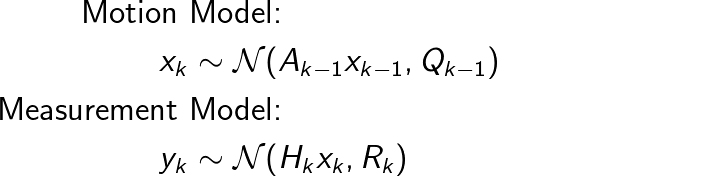
We have some knowledge of the dynamics of the airplane between time-steps, which we represent as a motion model. However, there is uncertainty in the model, which is why we view it as a probability distribution

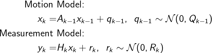
Expressed in words, the model says that the state x_k is drawn from a distribution over possible values of x_k, and that this distribution depends on the previous state x_{k-1}. We can also choose to express the motion model as

This equation says the same thing, but in this formulation we a deterministic function f() and a random variable q_{k-1}. So, expressed in words we have that the state x_k is a function of the previous state x_{k-1} and some random motion noise q_{k-1} which is stochastic (i.e. drawn from some distribution).

In addition to the dynamics of the airplane we also know the dynamics of the radar, which we can express as a measurement model. The sensor isn’t perfect, so we’re going to have noise in the measurements y_k that we receive. Because of this we can view the measurement model as a probability distribution as well

Expressed in words, the model says that the measurement y_k is drawn from a distribution over possible values of measurements y_k, and that this distribution depends on the state x_k. We can also choose to express the measurement model as

In this formulation we have a deterministic measurement model h() which receives the current state x_k as well as a random variable r_k. This says that the measurement y_k is a function of the state x_k as well as some stochastic (i.e. drawn from some distribution) measurement noise r_k.

We’re looking for a way to combine these two models, so that when we observe measurements from the radar we can formulate the following density

which is called the posterior distribution over the state, and can be seen as describing a region of plausible values for x_k, given all of the values that we have observed so far.

We can express this density by computing two equations, the predict and update equations

The predict equation uses the posterior from the previous time-step k-1 together with the motion model to predict what the current state x_k will be. This belief is then updated via the update equation by using Bayes’ theorem to combine the observed measurement y_k with the measurement model and the predicted state. We then end up with the posterior distribution! For the next measurement we just repeat these steps, and the current posterior becomes the previous posterior instead.

Alright, I’m up to speed now. So, what’s a Kalman filter?

The predict and update equations provide a recursive way to compute the posterior of the state for every measurement that we receive. However, if we look at the equations, they aren’t all that easy to compute in practice.

For starters, we need to express densities in such a way that we can actually solve the equations (i.e. we want numerically stable equations). Secondly, it would be nice if we could find analytical solutions, since then we wouldn’t have to numerically solve the equations (which might require a lot of compute). Both of these are important, especially when you consider that a lot of sensors give you measurements at a rate of hundreds or thousands hertz. Since we don’t want to discard measurements, we need to find a way to compute both equations really fast.

This is where the Kalman filter comes in. The Kalman filter is built around one key concept

This reason for this is that Gaussian densities have a lot of nice properties:

If we draw values from a Gaussian and perform a linear operation (i.e. multiplication and/or addition), these values will still be distributed according to a Gaussian.
Another nice property with Gaussian densities is that they are self-conjugate. This means that if we have a Gaussian likelihood and a Gaussian prior then the posterior is guaranteed to be a Gaussian as well.
Finally, Gaussian densities can be described entirely by their first two moments: the mean and the variance.

If we look at the predict and update equations you can hopefully see how all of these properties might come in handy. By making every density a Gaussian each equation boils down to finding expressions for the corresponding mean and variance!

The linear and Gaussian motion and measurement models can be expressed as

Just as before we can choose to express both of these models as functions instead of densities

With these in place we can rewrite the predict and update equations where all the densities are Gaussians

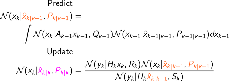
What we’re looking for is to find equations for how to compute the moments marked in orange and magenta above: the predicted mean and covariance, as well as the updated mean and covariance. I’m going to skip the derivations, but what we end up with is the following

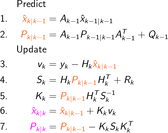
There we have it, we now have an analytical solution for computing the posterior distribution of the state x_k for every time-step! Since we end up with a Gaussian computing the MMSE or MAP is trivial, since the mean of the posterior serves as both. Another way to view it all is as the following

“The posterior (magenta colored) mean is the optimal estimate of the state, and the posterior (magenta colored) covariance is the uncertainty of the estimate”.

Before we move on to a practical example let’s take a brief look at each line and break down what’s happening.

We get the predicted mean by taking the past posterior mean and multiplying it with the matrix A_{k-1}, which makes sense since A_{k-1} describes how the state evolves over time.
The predicted covariance is computed in a similar manner, where we multiply the past posterior covariance with A_{k-1} twice and add Q_{k-1}. We add the covariance Q_{k-1} since we have uncertainty in our motion model, so that’s added to the transformed covariance.
v_k is called the innovation, and can be seen as a representation of the new information that’s gained when comparing the real measurement with the predicted measurement that we get from the measurement model.
S_k represents the predicted measurement covariance. R_k represents the measurement uncertainty in the measurement model, and with S_k we combine the uncertainty of the predicted state with the uncertainty of the measurement model.
K_k is called the Kalman gain and represents how much the predicted state and covariance should be adjusted with the new information gained from the measurement.
The posterior mean is computed by taking the predicted mean and adjusting it with the new information that has been gained. As noted in above, K_k is a scaling factor that determines how much of v_k should be added.
The posterior covariance is computed by taking the predicted covariance and adjusting it with information gained from the measurement. The new information allows us to decrease the uncertainty regarding the state, that’s why there’s a minus sign.

Yeah math is nice but I’m still kinda lost…

In order to understand a bit better what those 7 lines of equations represent it’s helpful to visualize on a conceptual level what’s going in a Kalman filter.

To start, we can image that we have two different planes (or dimensions): the measurement plane (red, denoted with Y) and the state plane (blue, denoted with X). The state x_k evolves over time in the state plane. The issue is that we can’t access or explicitly observe the state plane in any way, we only have access to the measurement plane. The measurement plane is where we observe measurements, which are caused by the state.

We can’t know for sure what’s going on in the state plane (i.e. we can’t observe an exact value of the state), but with the Kalman filter we can describe the state’s behavior in the state plane as a Gaussian density.

In the Kalman filter we start with an initial Gaussian, describing the state at time-step k-1. This initial Gaussian is illustrated with a black point and circle (the point represents the mean and the circle is a contour line of the covariance matrix). We use the motion model to predict where the state will be at time-step k, illustrated by the Gaussian in blue. We then use the measurement model to project the predicted state (blue Gaussian) from the state plane into the measurement plane. What we end up with is the red Gaussian, which essentially describes where we can expect the measurement to occur. Once the measurement is observed (indicated in green), we use the red Gaussian to decide how much of the measurement should be used to update the predicted state in the state plane. After we’ve updated the predicted state, we end up with a new black Gaussian, describing the posterior of the state at time k. This process is then repeated for all future time-steps.

Okay cool, how do I use this in practice?

Alright, let’s put all of this into practice by showing what a Kalman filter looks like in code and apply it to a toy example.

In the toy example we’ll use the airplane example that I mentioned before. To make things easy, let’s assume that the airplane is flying at a constant altitude. So, in this case we can choose to include xy-position as well as xy-velocity in the state

The motion of the airplane can be described by a constant velocity (CV) model. The CV model is nice since it’s a linear and simple model to implement and at the same time it manages to give quite a good representation of how an airplane behaves. Simply put, it assumes that the airplane’s next position is a function of its current position and current velocity. The velocity is assumed to be stochastic (subject to additive gaussian noise), which makes sense since we don’t know what actions the pilot is taking. In 1D this model is formulated as

The parameter T denotes the sampling-time that’s used in the system and σ² is used as a scaling factor for the covariance matrix (i.e. indicating how much uncertainty we have in the model). Now, the reason why the covariance model looks so funky is because we’re using a discretized CV model (read this for more info). This is important since our choice of sampling-time T will affect filter performance (I’ll go more in depth on this topic in a later post).

In our case where we have motion in both x and y directions, the motion model becomes

The 1D covariance components Σ for each direction are subscripted with x and y respectively. This is since both directions don’t necessarily suffer from the same amount of noise.

Okay so now we know how to formulate A and Q. Let’s go on to the measurement model. Now, this model is fairly simple. We assume that we measure the position of the airplane at every time-step and the measurements are stochastic (subject to additive gaussian noise). This can be expressed as

Similar to before we use λ² as a scaling factor for the measurement covariance matrix R_k.

Before we move on to implementing a Kalman Filter for this system we’ll use these two models to generate motion and measurement data. We’ll use this data later on to test out the Kalman Filter and see how well it works. For this we’ll need a script that can simulate the system and create all of the model parameters (Note that the @ operator is the same as np.matmul in numpy, so A @ B is the same as np.matmul(A, B)).

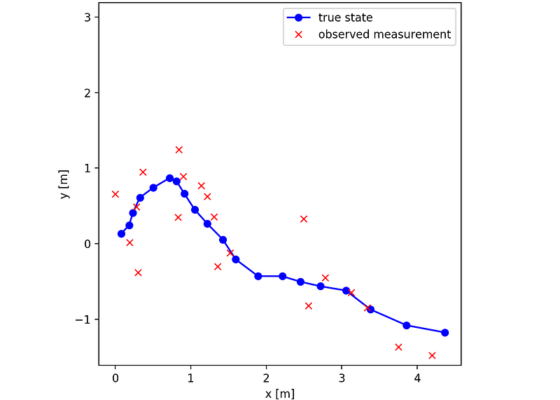
After running simulate_model.py we get the following plot, illustrating how the positional components (x and y) of the state evolved over 20 time-steps (with sampling time T=1), as well as the measurements that were observed. Now keep in mind that we’re simulating the system, that’s how we know what the true state is.

Now let’s implement the Kalman filter, which is a straightforward process since the filter equations translate from math into code really easy.

With the Kalman filter in place we can now run it and see how it performs on our simulated data. In order to do this we’ll write a script that combines the functionality found in kalman_filter.py and simulate_model.py.

After running the script we get the following plot, which is the same as the one before but with the addition of the Kalman filter’s estimate of the x and y positions.

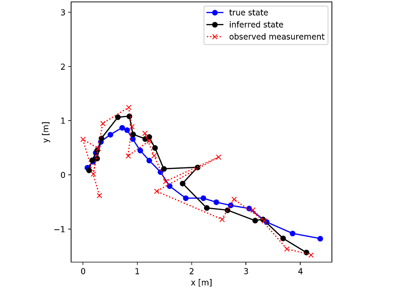
Just by looking at the plot it’s clear that the Kalman filter gives better estimates of the x- and y-position than if one were to just use the raw measurements. The superior performance of the Kalman filter to that of just using measurements can also be analyzed numerically. By using euclidean distance as error metric for the x- and y-position we can compute the Root Mean Square Error (RMSE) for both the Kalman filer and the measurements. For this 20 time-step long scenario the RMSE for each method is

(20 time-step simulation)
RMSE Kalman Filter: 0.2917
RMSE Measurements:  0.4441

The Kalman filter has a lower RMSE value than the measurements by quite a large margin. Since 20 time-steps is pretty short so let’s investigate if the RMSE results hold for a longer simulation less prone to statistical uncertainty.

(100,000 time-step simulation)
RMSE Kalman Filter: 0.3162
RMSE Measurements:  0.4241

Just like before the kalman filter a better option than just using measurements.

(The comparison has only focused on the positional states, since these are easier to plot. But don’t forget that with our chosen motion model we’re also getting estimates of the x- and y-velocities as well from the Kalman filter!)

It’s important to stress that the purpose of the toy example is to illustrate how the Kalman filter works. In real world applications we don’t know the model parameters beforehand (Q and R) and we might not even know what motion model to use. In such cases a lot of time is spent tuning the filter parameters and trying out different motion models. To make matters worse, most of the time we end up dealing with systems that are nonlinear and where the Gaussian assumption doesn’t hold.

But at the same time, it’s these types of problems that are actually the most fun to solve! This is where the more complex variants or extensions of the kalman filter come in — they provide different methods and strategies to address either all or some of these issues, depending on the need.

In the next post of this series I’ll explore the family of sigma-point filters, which consist of several different filters capable of tackling nonlinear and non Gaussian models to varying degrees.

Thanks for reading!