

Word Vectors and Lexical Semantics — Introduction to Count-based Vectors
The following are my personal notes based on the Deep NLP course by Oxford University held in 2017. The material is available at [1].
Introduction
Word Vectors : Representation of word in vector format.
Lexical Semantics : Analysis of word meanings and relationship between them.
Neural network requires vector representation as inputs. Thus there is a need to change words or sentences into the vectors.
Representing Words
Text are merely sequences of discrete symbols (i.e words). A simple way to represent them is by one-hot encoding every words in the sentence. However doing this would require a lot of memory/space as the vector space (made up of one-hot encoded vectors) would effectively be the size of your vocabulary.
The problem with this approach is since each vector is defined a single word, every vectors are then represented in a rather orthogonal way without no clear (weak) relation to each other in terms of semantics. They are also very sparse from each other. Thus there is a need for richer representation which is able to express semantic similarity.
Distributional Semantics
Distributional Semantics : A research area that develops and studies theories and methods for quantifying and categorizing semantic similarities between linguistic items based on their distributional properties in large samples of language data [2].
“You shall know a word by the company it keeps” — J.R Firth (1957)
The above quote, and other analogies similar to it — points out that meaning of words can be understood by looking at how it is being used by the population.
At the same time, we are also interested in reducing the size of our vector space. This can be done by producing dense vector representation (as opposed to sparse).
Computationally, there are 3 main approaches to doing this.
- Count-based
- Predictive
- Task-based
The advantage of being able to assign words as vectors is that one can start to objectively measure and compare between the word vectors, either to calculate similarity, distance and others.
Let’s cover the count-based method first.
Count-based Method
Define the basis vocabulary to be used. Usually they’re chosen based on our own experience/intuition or statistics of the corpus. These vocabulary ideally is informative and has meaning.
Usually the size of the vocabulary will be limited. Stop words are typically excluded since they appear a lot in most available corpus. If we’re to include them, then we’ll have trouble identifying relationship due to the co-occurrence of the stop words all over the place.
Let’s look at an example:
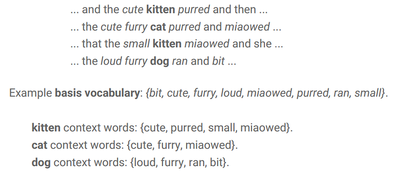
In the above example, we can see that certain words have been chosen as the basis vocabulary that we’re interested in. Notice also that stop words like “and”, “the” and “that” are not part of the basis vocabulary.
Having identified the target words and it’s context, we can now represent this as a vector (as below).
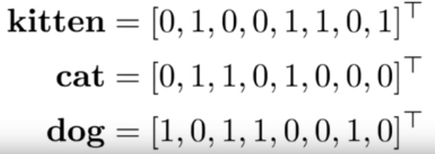
As vectors, the words can now be analyzed, perhaps via similarity (most popular method to calculate similarity is cosine distance), distance in vector space and others.
However, there are still some disadvantages:
- Not all words are equally informative, since some words can simply appear more frequently in the various texts; and by virtue of that, can no longer be uniquely associated to a particular context.
- For example, in texts that describes various 4 legged animals — the word run or four legs wouldn’t be able to differentiate the types of animal within the corpus.
- They are methods however to overcome this, like TF-IDF or PMI.
In my next post, we’ll explore an easier way to resolve these issues.