Why you Should Stop Predicting Prices if you want to Stand a Chance of Predicting Prices

Financial Data Almost Might have been Designed to Beat You

The internet is full of forums, such as Towards Data Science here on Medium, that are full of eager articles explaining how to use today’s modern “AI” tools to predict stock prices. I find the articles they publish follow a common pattern:

1. The author provides code snippets, almost exclusively in Python, that shows how to pull data from free public data sources, such as Yahoo! Finance or Quandl, using a simple API.
2. They then include some commentary on how advanced and complex neural networks, such as LSTM networks, are “known to be accurate” when predicting time-series, and dive into their theory and structure.
3. Next they demonstrate how to train these networks, using popular open source frameworks, and claim a high accuracy on the training set, such as 85% or more.
4. Finally the system is run out of sample and draws a curve which kinda looks like a moving average over the prices of, say Tesla or IBM, but, truth be told, basically sucks as a forecast of the stock price.
5. In conclusion, they state that the performance is “not so bad” and the system needs “more work.”

When these posts appear in my feed, here on Medium, I sometimes add a comment along the lines of:

Did you compare your model’s performance to just using the last price?

Martingales

What is a Martingale?

A “martingale” is a strap that is attached between the bottom of the bridle of a horse (the harness around it’s head) and to one that passes around it’s chest. It’s purpose is to hold it’s head down. It is also the name of a betting strategy, apparently popular in France around the 18th. Century, which involves doubling your stake every time you lose. Some simple math leads to the (false) conclusion that you cannot lose, but people who play the martingale are well known to regularly ruin themselves.

The martingale strategy stimulated mathematical work to address the following interesting question:

In a fair game, is it possible to arrange your sequence and size of bets so that you can generate wealth with certainty?

TL;DR? The answer is no! This seems like a reasonable answer to me. Otherwise mere paper accounting could be used to create a magic money machine. Why is this so? The answer lies in a thing called The Optional Stopping Theorem, which describes many things including playing the martingale on a fair game.

As a side note, it’s called a “theorem” because it is something that has been rigorously proved to be true within the analytical framework that describes probability. You can’t argue with it, it’s as true as Fermat’s Last Theorem.

The O.S.T. says that if you play the martingale on a fair coin flipping game that is either finite in length (fixed number of flips), or that ends with your bankruptcy (fixed bankroll), then the expected value of your final wealth is equal to your initial wealth.

We write that

meaning that the expected future value of the wealth, W, equals the current value: you cannot, on average, make money from this strategy.

Mathematicians, and sophisticated finance types, have subsequently decided to label all time series with this property as “martingales.” For people like me, involved in forecasting the futures values of asset prices, it is also known as the “naive forecast,” the “baseline forecast,” or, sometimes, the Bayesian Prior for the future price, as it is the assumption that, at sometime in the future, nothing has changed. The martingale should be a baseline forecast for any time-series method. If you can’t beat it, you are subtracting value.

The quality of a forecast is often measured in terms of “forecasting skill,” defined to be

and the baseline should be the martingale.

Stock Prices are Very Close to Martingales

If you want to demonstrate to yourself that stock prices are very close to martingales an easy way is to head over to Google Research’s Colabatory and play with some data.

To start off, you can bring in the popular yfinance package

!pip install yfinance

and then get some data. For tradition’s sake, let’s get IBM’s stock price:

from yfinance import download
ticker='IBM'
df=download(ticker)
plot=df["Adj Close"].plot(label=ticker)
plot.legend(loc="best");

You should get a chart that looks like this

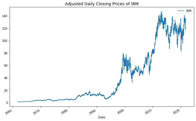
which shows the “adjusted” daily closing prices of IBM. That means prices that have been changed to reflect any stock splits, spin-offs, mergers, and capital distributions that may have occurred over time. Such things generally generate discontinuous jumps in the price which do not reflect real returns, as the shareholder would receive the value distributed in the change.

Now make a second time-series that is the price of IBM lagged by just one day. This is the prior day’s closing price that you could use to predict the today’s price before the end of the day if the price of IBM happened to be a martingale.

df["Lagged"]=df["Adj Close"].shift()
df[["Adj Close","Lagged"]].plot();

You should get a second plot, that looks like this

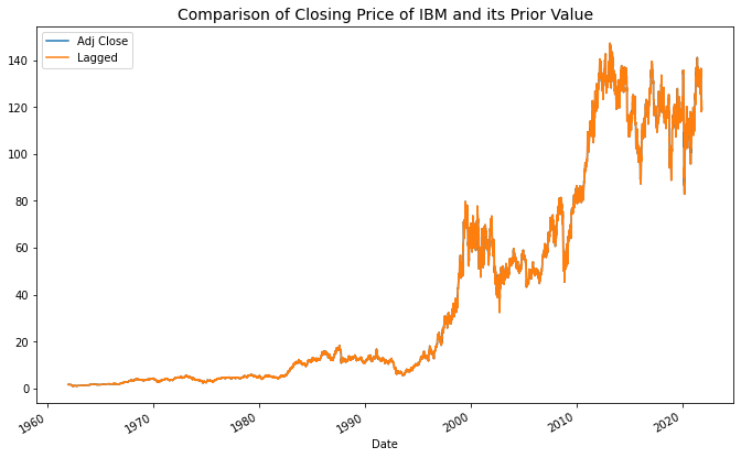
The striking fact here is that you can barely see any difference between the two time-series. They seem to be very similar, so let’s do a quick check via the correlation coefficient.

vcv=df[["Adj Close","Lagged"]].corr()

If you do this you’re going to find that the correlation between the two series, ρ, is extremely high (99.98% at the time of writing). That is equivalent to an R² in a linear regression model of ρ², or 99.96%. That’s an almost perfect model, arrived at trivially.

import numpy as np
print("R2 of %6.3f%%" % (
    np.power(vcv.loc["Adj Close","Lagged"],2)*1e2))

Let’s find out how statistically significant the result is. The quick’n’dirty way to do that is to compute the sampling error of the correlation coefficient, which R.A. Fisher showed was approximately given by

for a sample of size N. For our data we get

1e0/np.sqrt(df.dropna().shape[0]-3e0)

which produces a value of 0.8%. Take a look at that again, the standard error for a correlation coefficient is 0.8% when the null hypothesis value is ρ=0 and the measured value is 99.98%.

The martingale is a very tall hill for a forecasting algorithm to die on.

The Martingale Forecast is Not Useful

Unfortunately, this martingale forecast is not useful. It’s an observed or stylized fact, as they say in finance, that prices do change and, if you try to make money from this, you won’t get anywhere. You need to predict the difference between yesterday’s price and today’s, that prediction needs to be non-zero, and you need to make that prediction yesterday.

Curve Fitting with Martingales

Linear Regression and it’s Cousins

Linear regression was invented by Gauss, potentially the most brilliant mathematician of his time and maybe our time, to fit curves to astronomical observations. Laplace also worked on this problem and, interestingly, he proposed minimizing the absolute deviation of the errors but that was not analytically tractable. Gauss introduced the mean squared error and deployed the methods of geometry and calculus to deliver an answer.

I’m going to assume my readers are familiar with the linear regression equation, which posits that an observed variable, y, is linearly related to a predictor variable, x, with additive noise, ε.

Built into this expression is an assumption, and that assumption can make linear regression, and its cousin non-linear regression, go really wrong when applied to time-series that are martingales, or close to it.

Independent Variables

Performing an experiment is supposed to be a clean discipline:

1. We chose values of a predictor variable, which we call independent, and use it to probe our response variable, which we call dependent.
2. We write down these pairs of data, and turn the handles of Gauss’s remarkable machinery, and it tells us which values to use for the unknown coefficients, α and β, in the relationship.

We are using x as a probe to discover the response of y to it’s variations.

Dependent Variables

What we’ve done here is to assume that the variation of y is entirely governed by the variation of x and some additional random noise. We also have taken no account of the dependence of x and y on prior-values of themselves and we have assumed that x is a probe under our control. If x and y are observed financial time-series, though, this is not true.

Unfortunately, the whole framework fails when we try to apply it in a time-series context with martingales. Suppose

These series are both martingales, and are also known as random walks because their ultimate value is a function of the sum of independent random numbers.

Making Martingales

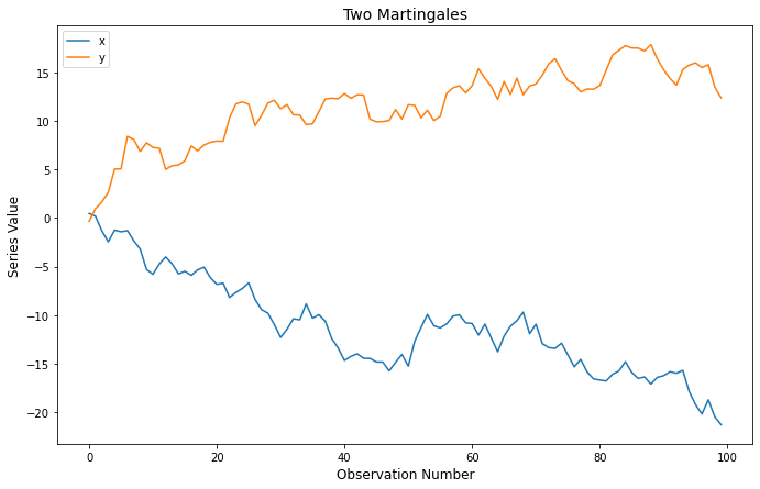
Let’s take the time to build two such series, so we can see what’s going on in more detail.

import numpy as np
import pandas as pd
npts=100

# so the plot is repeatable, I'll set a random seed
# and this is not a "mined" seed, as is clear from it's value
np.random.seed(123456)

df=pd.DataFrame({
   'x':np.random.normal(size=npts),
   'y':np.random.normal(size=npts)
})

for column in df:
    df[column]=df[column].cumsum()

plot=df.plot()
plot.set_title("Two Martingales");

This is very easy, and the data look like this:

Regression with Martingales

If we try to perform a regression of one series on the other we sometimes will find a significant relationship but we know, by construction, that there is absolutely no predictive power in this because the future values of the series are entirely random.

Nevertheless, let’s do it:

from statsmodels.formula.api import ols
from statsmodels.sandbox.regression.predstd \
    import wls_prediction_std

alpha=0.05 # set alpha_critical to 5%
fit=ols("y ~ x",df).fit() # do OLS regression
df['yhat']=fit.fittedvalues # get the fit
print(fit.summary()) # print the regression summary

That’s pretty easy, thanks to the statsmodels package. The results are:

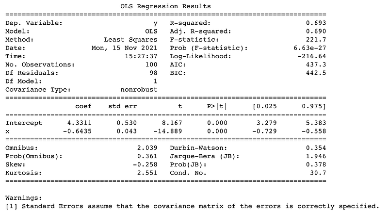
This is a massively significant regression, which means there is a strong relationship observed between the historic values of the two series. However, that relationship must have occurred by chance, by construction.

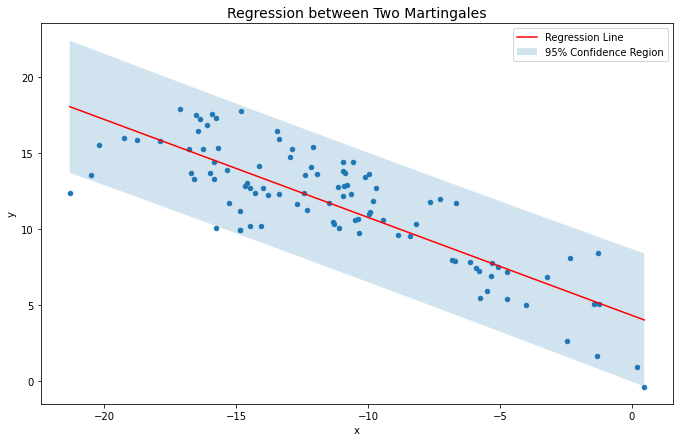
There is no real relationship between these series, but regression analysis doesn’t seem to agree with that.

Here’s the code that makes the plot…

plot=df.plot.scatter("x","y")

# get the raw data
x,y,yhat=tuple(map(lambda c:df[c].tolist(),list(df)))

# get the confidence regions with given alphasig,crl,cru,=wls_prediction_std(fit,alpha=alpha)

# sort all values by x
x,y,yhat,crl,cru=tuple(zip(*list(sorted(zip(x,y,yhat,crl,cru),
                                        key=lambda a:a[0]))))

plot.plot(x,yhat,'r-',label='Regression Line')
plot.fill_between(x,crl,cru,alpha=0.2,
    label='%.0f%% Confidence Region' % (1e2-1e2*alpha))
plot.legend(loc="best");

A Monte Carlo Experiment that Shows that Statistics is Broken?

The significance of a regression is usually judged by a statistic called F, after R.A. Fisher. The specific value of F is weighed by its p value, which is the probability of getting a larger value by chance if the data are completely unrelated. It’s the false positive rate for this analysis, and we can compute its distribution by making a few thousand simulations.

It’s trivial to generate thousands of pairs of time series, x and y, and regress them onto each other. The following code runs 1,000 regressions on randomly generated pairs of data:

f_stats=pd.DataFrame({'F':[],'p':[]})

for i in range(1000):
    df=pd.DataFrame({
        'x':np.random.normal(size=npts),
        'y':np.random.normal(size=npts)
    })

    for column in df:
        df[column]=df[column].cumsum()

    fit=ols("y ~ x",df).fit()
    f_stats=f_stats.append(pd.DataFrame({
        'F':[fit.fvalue],
        'p':[fit.f_pvalue]
    }))

It’s easy to then make a histogram of this data but, before doing that, let’s work out what to expect. The data series are 100 points long and there are two regressors, one of which is the mean and the other the independent variable, so under the null hypothesis of no relationship between y and x, the F statistic we are computing should be drawn from an F distribution with 1 and 98 “degrees of freedom.” These are the parameters of the distribution, and the mean is determined by the second value: it is the ratio of that value to itself minus two. Thus we expect this distribution to have a mean of around 98/96 ≈1.02.

The shape of the F distribution is perhaps a little less familiar to many, but we should also expect around 5% of our regressions to have a significant p value by chance at the standard (but weak) confidence level of 95%. That much everybody should be familiar with. However, we know even more than that about the distribution of p for our experiment. Since p is a cumulative probability

then p itself should have a Uniform distribution on [0,1]. It clearly doesn’t!

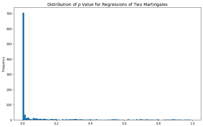
figure,plot=pl.subplots(figsize=figure_size)
f_stats['p'].plot.hist(ax=plot,bins=np.linspace(0,1,100))
plot.set_title("Distribution of $p$ Value for Regressions of Two Martingales",fontsize=14);

Is the Science of Statistics Broken or Useless?

That histogram is going to give us many-many false positives, many more than we should have based on regression theory, and we know absolutely none of them are significant because the series we have created are definitely not related by virtue of the way they’re constructed.

So what’s happening here is that we are violating the assumptions upon which linear regression is built by using it on martingales not on data with measured values that are independent of each other.

Saving Statistics through Differencing

We can recover everything we need to make our statistical analysis accurate by taking account of the integrated nature of these time series. Let’s take look at the relationship of their differences

There clearly should be no dependence of Δy on Δx, and and regression tells us there is not.

for column in df:
    df["Δ"+column]=df[column].diff()

fit=ols('Δy ~ Δx',df).fit()
print(fit.summary())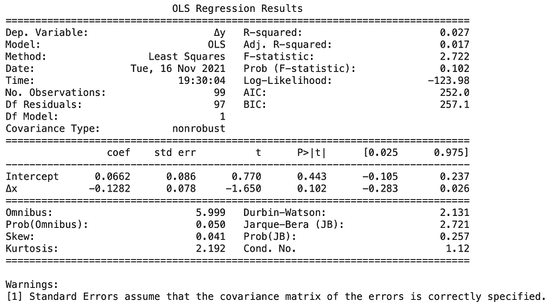

Financial and Economic Data are Close to Martingales

We’ve seen in this article that the price of IBM stock is very close to a martingale, and probably well described by that model to first order. This is true of many stocks and many economic time-series. Taking data that might be martingales and attempting linear regression on them will lead to models that seem to work on historic data but actually don’t possess any useful predictive value.

It doesn’t matter whether you have a good in-sample/out-of-sample division of your data and it doesn’t matter if you do five-fold cross-validation or ten-fold cross-validation or whatever is taught in data-science boot camps. This analysis will fail.

The relationship between the data that you see is a true relationship between historic data, albeit one that occurred by chance, and not a predictive relationship of use in the future. Statistics works, but if you are asking it the wrong question you will not get a meaningful answer.

The observed historic relationships between financial and economic time-series are real, but often not of predictive value.

How to Build Models that Work

Differencing Away the Integration

The random walk model we’ve used has another name, it’s called an integrated moving average model or IMA(1,1). That’s because it can be viewed as through Box and Jenkin’s ARIMA framework as having one “integration” step and one moving average lag. The ARIMA(p,d,q) model is

which states that a polynomial in the lag operator, L, of order p, applied to the data after d stages of differencing, is equal to a polynomial in L of order q applied to the random noise innovations. The “lag operator” sounds fancy, but it just shifts the time index by one, very much as .shift() does in Pandas. The differencing can be expressed in terms of it as well.

Testing for Integration

One of the key signatures of “integration” in a time-series is extremely high first lag autocorrelation. There are many ways of looking for this, but the most widely used is the Augmented Dickey-Fuller Test. You can, and should, apply this to a time-series before you start using it in a regression analysis. That way you’ll get more reliable results and not produce complicated models that underperform the “no change” forecast that requires no effort to compute.

If you like this article and would like to read more of my work, consider my book Adventures in Financial Data Science which is available as an eBook for Kindle, and also from Apple Books and Google Books. A revised second edition will be published by World Scientific.

Alternatively, you can order the paperback directly from me via our website.

You can directly support my writing on Medium by subscribing through this affiliate link.