Making Sense of Big Data

Why you should not rely on t-SNE, UMAP or TriMAP

Use PaCMAP instead for increased interpretability & speed

Dimensionality reduction techniques such as t-SNE¹, UMAP², and TriMap³ are ubiquitous within the field of data science, and given their impressive visual performance (combined with ease of use), they can therefore rightfully be found in any complete exploratory data analysis of a given dataset. However, these specific methods (t-SNE, UMAP and TriMAP) likely should not be your first go-to option for dimensionality reduction . In this post I will go over why, as well as suggest a recently published alternative from 2020 that is more interpretable, results in higher quality results, runs faster, and requires less manual tuning — all the good things 👍 🍾

Before we start, I’ll note that I myself have been (and still am) an avid user of both t-SNE, UMAP and TriMAP. Sadly, the technical details of the inner workings for these techniques is often neglected, especially by less experienced practitioners, which has consequences for the interpretation of visual results. Specifically, it is important to be aware of the trade-off each algorithm makes in terms of retaining global vs. local structure. Beyond interpretation issues, often-used implementations of e.g. t-SNE (as in scikit-learn) can be annoyingly slow, resulting in the waste of a lot of time setting up the algorithms, potentially fine-tuning them, and finally running them over and over as people constantly restart their everything_in_here.ipynb notebooks. Finally, and maybe most importantly, a lot of the algorithms can be tuned to make super impressive visuals in tutorial-settings when we already know the final labels (e.g. as for typically shown benchmarks such as MNIST, Cifar10, etc.), but when using it in real life on an unknown dataset, then it is far more difficult to know how to interpret a given visualization, because we do not necessarily know a whole lot about the dataset beforehand — here an algorithm that by default more often gets it “right” the first time, is definitely an advantage.

In this post the intuition underlying various dimensionality reduction techniques is briefly reviewed, and then a more recent algorithm PaCMAP⁴ is introduced and reviewed. This new algorithm manages to improve on the global vs. local trade-off, does well without parameter tuning, is fast, and easy-to-use. The hyper parameters of the algorithm are furthermore very intuitive, and can be used to smoothly transition between a focus on local to global structure. I am not advocating abandoning methods such as PCA, t-SNE, UMAP, TriMAP etc, but for most intents and purposes, I think algorithms such as PaCMAP should be your first choice, especially if you are a newcomer or are in a hurry.

PS. I have no relation to the creators of PaCMAP, but I highly recommend you go read their paper for an even more in depth introduction!

Dimensionality reduction methods

Reducing the dimensionality of a high dimensional dataset (e.g. if we have >3 columns in a tabular dataset) allows us to potentially get an increased understanding of underlying clusters in the dataset, or get an intuition for the distribution of the data (useful e.g. for comparing training & test datasets). The goal is to retain as much “structure”/information in the data as possible, so that points which are far away from each other in the original high-dimensional space are also far away in the low-dimensional space, and vice versa for points close to each other. Overall, these algorithms can be split into two primary archetypes; those that aim to preserve local structure (observations very similar to each other) and those aiming to preserve global structure (observations very dissimilar to each other).

It is known that visualized projections created with these algorithms can be misleading, e.g. reflecting clusters that do not exist or insinuating that clusters are close to each other, even though they are not. It is therefore a good idea to be very conservative in the interpretation of any projections made with a dimensionality reduction algorithm as well as have an understanding of the algorithm itself. In the following the intuition for a few well-known algorithms is briefly reviewed.

PCA: here the data (which is potentially correlated) is reframed into uncorrelated principal components, which contain decreasing amounts of information as measured by variance. Using this method to visualize only the first initial components (describing most of the variance) is inherently a method that captures primarily the global structure of the data.

t-SNE: here gradient descent is used to find a low dimensional embedding in which a relative distance between point i and j match that in the original high-dimensional space, under the control of a not very intuitive perplexity parameter that determines the standard deviation of the conditional distributions used for the relative distance calculations in high-dimensional space. This method primarily focuses on local structure, in that it puts focus on nearest neighbors in the relative distance calculations.

UMAP: here a weighted graph of nearest neighbors is constructed with vertices being observations / data points, and stochastic gradient descent is then used to optimize a lower-dimensional graph to be as structurally similar as possible to the high-dimensional one. UMAP has a lot of advantages over t-SNE in that it better preserves global structure, is faster, and has slightly more interpretable hyper parameters, but at its core it uses distances between nearest neighbors in the construction of the graph, and as such focuses on local structure.

TriMAP: here triplets (sets of three observations) are created predominantly from nearest neighbors, but with a fraction of the triplets also containing one or two randomly sampled points. The algorithm then tries to find a lower dimensional embedding using batch gradient descent, which preserves the ordering of distances of the triplets. Theoretically this method manages to include both local and global structure, but in practice it is typically found to be prone to struggle with local structure.

Introducing PaCMAP

In the PaCMAP paper they show that methods such as t-SNE, UMAP and TriMAP all can be viewed as graph-based algorithms with nodes being observations and edges constituting a similarity metric between these observations — given a high-dimensional graph, a loss function is defined and optimized to find a low-dimensional representation of the graph that is structurally similar. With this insight, firstly they investigate the loss functions of known algorithms as well as various dummy loss functions, and from this are able to deduce several key principles which make for the “ideal” loss function (section 4 of the paper). Secondly they investigate how to optimize the low-dimensional graph in a way to conserve both local and global graph structure, again showing how most algorithms are near-sighted (i.e. focus on local structure). The authors suggest a method of using mid-near pairs of observations as well as a dynamic choice of which graph elements are optimized during the convergence, such that the algorithm initially gets the global structure right, and subsequently refines the local structure (section 5 of the paper).

The combination of the choice of a better loss function as well as the suggested graph optimization technique constitute the new method PaCMAP, which the authors show have good performance both on local and global structure. Furthermore they show that the suggested algorithm is quite robust to initialization, and works well on the chosen datasets by using default hyper parameters, while being significantly faster than the fastest other algorithm on all 11 tested datasets.

Comparing results

Let us re-run some of the experiments from the papers, to compare results between a few algorithms. Running PaCMAP is just as easy as running any other dimensionality reduction algorithm — in my own comparisons, I tested algorithms from following PyPi packages: t-SNE from scikit-learn==0.24.1, UMAP from umap-learn==0.5.1, TriMAP from trimap==1.0.15, and PaCMAP from pacmap==0.3. To create my embeddings I used the following small snippet — the main point here is that I use all default settings and no tuning.

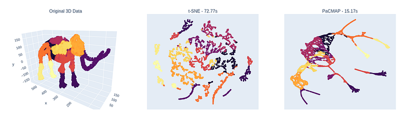
In the paper they have a nice visualization where they use different techniques to reduce the 3D representation of a mammoth to 2D. Trying to re-create that, I got the following result with all default hyper parameters:

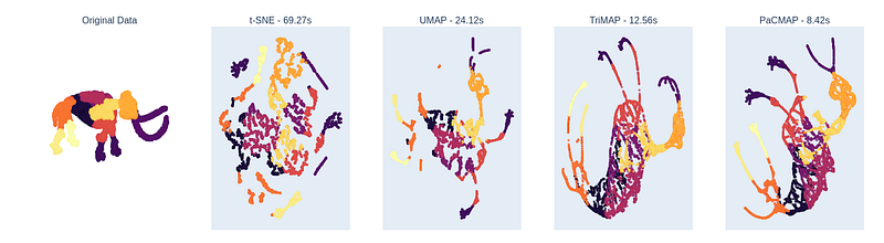
It becomes very clear that t-SNE, at least with default parameters, focuses primarily on local structure, UMAP captures the global structure a little better, TriMAP does a decent job of global structure, but fails on local structure (see feet & horns), while PaCMAP seems to capture both global and local structure. At the same time, PaCMAP finishes in only 8.4 seconds, faster than TriMAP at 12.56 seconds, UMAP at 24 seconds, and t-SNE at 69 seconds.

Stress-testing the algorithms a little more, I performed the same test on the classic MNIST dataset with (60,000 train images, 784 pixel columns). Results were as follows, again with all default hyper parameters:

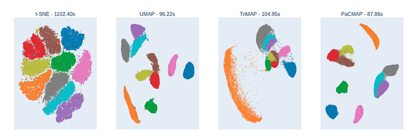
Here we see that t-SNE distributes the clusters uniformly around the center, which probably contributes towards preserving local structure, but seems not to contain much information about the global structure — in addition we see that the algorithm actually also seems to identify some wrong clusters (the red, brown and purple ones, which we only ‘know’ because we have those labels). Again, these results are consistent with what was seen in the PaCMAP paper, indicating that t-SNE & UMAP focus primarily on local structure, TriMAP on global, and PaCMAP on both.

These two examples match pretty well what was shown in the PaCMAP paper — I encourage everyone to go read the paper to see additional examples, quantifications, and interpretations.

Conclusions

As stated initially I am not advocating abandoning PCA, t-SNE, UMAP, TriMAP etc. However, time is often of essence, and as such I believe that PaCMAP provides two pretty major benefits; 1) both local & global structure is captured by default, and it is easy to change the focus between local and global structure with hyper parameters if needed, and 2) it is faster. These benefits are especially important in cases where dimensionality reduction is not the core part of an analysis and you do not have time to thoroughly investigate a multitude of hyper parameters, algorithms, etc.

A complete analysis should include multiple algorithms and hyper parameters, while ensuring that it is possible to explain the differences between each experiment based on knowledge about the specific algorithms.

Finally, kudos and thanks to the writers of the PaCMAP paper.

[1] Laurens van der Maaten & Geoffrey Hinton, Visualizing Data using t-SNE (2008), Journal of Machine Learning Research 9, 2579–2605

[2] Leland McInnes, John Healy, James Melville, UMAP: Uniform Manifold Approximation and Projection for Dimension Reduction (2018), https://arxiv.org/abs/1802.03426

[3] Ehsan Amid, Manfred K. Warmuth, TriMap: Large-scale Dimensionality Reduction Using Triplets (2019), https://arxiv.org/abs/1910.00204

[4] Yingfan Wang, Haiyang Huang, Cynthia Rudin, Yaron Shaposhnik, Understanding How Dimension Reduction Tools Work: An Empirical Approach to Deciphering t-SNE, UMAP, TriMAP, and PaCMAP for Data Visualization (2020), https://arxiv.org/abs/2012.04456