

Why Random Forests can’t predict trends and how to overcome this problem?
Random Forests are generally quite immune to statistical assumptions, preprocessing burden, handling missing values and are, therefore, considered a great starting point for most practical solutions! While Random Forests might not win you a Kaggle competition, it is fairly easy to get into the top 15% of the leaderboard! Trust me, I’ve tried and won an in-class Kaggle Competition at General Assembly using Random Forests and it’s variant Extra Trees Classifier (which are highly randomised trees) with 87% ROC score which was 5% more than the 2nd place Winner.
While doing the Introduction to Machine Learning course from fast.ai taught by Jeremy Howard (whom I am an ardent follower of), I was introduced to the problem of Extrapolation in Random Forests. Jeremy claimed that Random Forests don’t fit very well for time-series data! Through this article, I share Jeremy’s teachings and explore techniques of solving the problem of Extrapolation in Random Forests.
But, I’ve only just recently started playing around with Time-Series data with Kaggle competitions such as Google Store prediction or Taxi Fare prediction and to my surprise, I have come across a drawback in Random Forests. Random Forests don’t fit very well for increasing or decreasing trends which are usually encountered when dealing with time-series analysis, such as seasonality! (If you are not aware of time series analysis, here is an article that might get you started)
Let me illustrate Extrapolation with the help of an example.
Let’s create a synthetic dataset for this purpose. (Note: When stuck, create a synthetic dataset and try things out for yourself! — Advise from Jeremy).
x = np.linspace(0,1, num=50)Let x be our input which is linearly distributed between 0 and 1, and is a Vector of size 50.
Let, our dependent variable ‘y’ be a Linear Function of ‘x’ with some random noise to add variance. The random noise somewhat mimics a real-world scenario.
y = x + np.random.uniform(-0.2, 0.2, x.shape)Let’s plot our X and y .
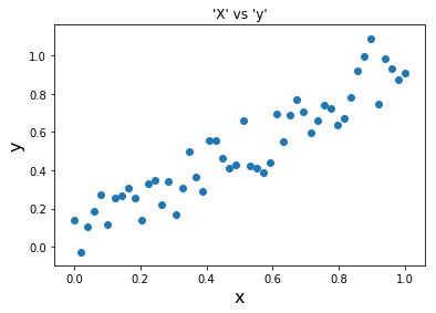
It is quite clear that a linear relationship exists between ‘X’ and ‘y’ and there is an increasing trend.
This can be very similar to a growing trend in a real-world use case— such as growing sales in the months of Oct, Nov, Dec or population growth in the world in 2019 etc.
Jeremy’s claim is that fitting a Random Forest on such a data won’t give us good results. So, let’s try and fit a Random Forests and see what happens!
X_train, X_val = x[:40], x[40:]
y_train, y_val = y[:40], y[40:]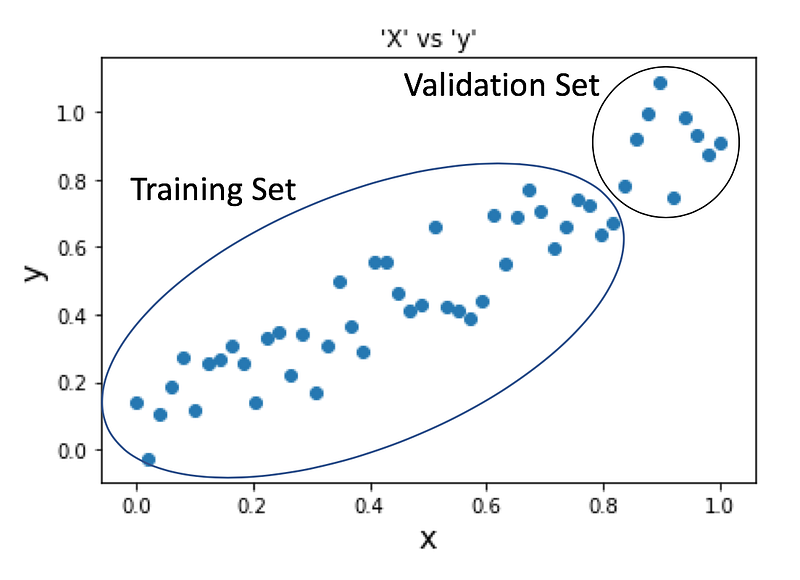
We will fit our Random Forest Regressor for training data and first explore how it goes with predicting X_train and then move on to X_val .
m = RandomForestRegressor(n_estimators=10)
m.fit(X_train, y_train)
m.predict(X_train)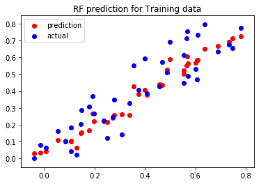
Our Random Forest seems to be doing really well for training data! (which it should be, it has seen this data before).
Now, let’s move on to the interesting part and predict X_val. Remember, our Random Forest has not seen this data before, what do you expect will happen when we predict validation data? This would be a good time to take a minute to ponder upon this question before scrolling down.
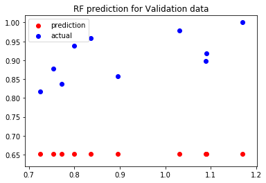
Our Random Forest is not able to predict for values that it hasn’t seen before! It predicts the Dependant Variable value of 0.65 for all validation data. Strange? Not quite.
Why are the predicted values significantly less than the actual values for our Validation set while it works perfectly well for the Training data?
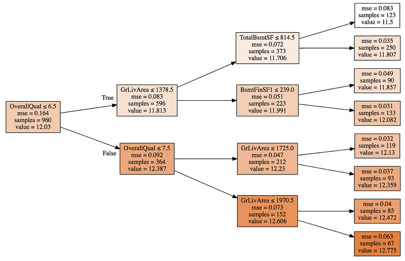
To answer this question we might have to take a deep dive into how Random Forests work. We will take help from Ames Housing data to explain the answer.
A Random Forest constitutes of Decision Trees (weak classifier) which in itself are a combination of Binary Splits (decision) on training data. Intuitively, you can think of this as a fancy way of grouping nearest neighbours. A Decision Tree brings together houses that might fall in the same price category, ie, it separates expensive houses from the cheap ones by grouping the houses. Houses with OverallQual ≤ 7.5 living area ≤1970.5 (67 samples/houses) are grouped together in the bottom-most leaf node. For any house in the validation set that falls in this leaf, the predicted value is the average value of the 67 samples, ie, 12.775.
For any data, that a Random Forest has not seen before, at best, it can predict an average of training values that it has seen before. It the Validation set consists of data points that are greater or less than the training data points, a Random Forest will provide us with Average results as it is not able to Extrapolate and understand the growing/decreasing trend in our data.
Therefore, a Random Forest model does not scale very well for time-series data and might need to be constantly updated in Production or trained with some Random Data that lies outside our range of Training set.
Answering questions like “What would the Sales be for next Year?”, “What would the population of China be after 5 years?”, “What would the global temperature be in 50 years from now?” or “How many units am I expected to sell for gloves in the next three months?” becomes really difficult when using Random Forests.
How to solve this Problem of Extrapolation?
- Look for other options
Therefore, fitting a Linear Model or a Neural Net, in this case, might be sufficient to predict data which has an increasing/decreasing trend.
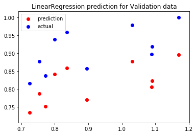
Here’s how the results look like when I fit a LinearRegression model on the same dataset. It would also be possible to fit a Neural Network which can be used for Demand Forecasting, or any other type of time-series plots. Stay tuned for another article on how to do demand-forecasting using Neural Networks.
2. Ignore the time-series components of data while training the Random Forest
This is a subtle one but another possible way to improve generalisation (we say a model generalises well if it predicts well for data it hasn’t seen before and a major challenge in Machine Learning is to create scalable and generalisable robust ML models) such that our model is able to predict for future data is to not use features in our data that might be related to time component. Our input matrix might have various features which are used to predict our dependent variable. If we do not use the time-related features for our predictions, our Random Forest model will be able to generalise really well!
Consider an example, the Bluebook for Bulldozers challenge on Kaggle, where the aim is to predict the ‘Price’ of heavy equipment in the future months. On checking feature importance for the competition, we get the following table:
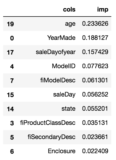
The most important features are Age, YearMade and SaleDayofyear which are all time-dependent! This might also be a good time to state the validation LRMSE score of 0.249366 with above feature importance.
What do you expect to happen to our validation score if we drop these time-dependent features? It goes down to 0.210967!
Our model generalises better and therefore, we see a reduction in the Validation Set Log Root Mean Square(LRMSE) error.
Further improvements: Another idea to further improve predictions using Random Forests is to use Time-Series forecasting to flatten the seasonality and then use a Random Forest to make predictions.


