Free AI web copilot to create summaries, insights and extended knowledge, download it at here

6469

Abstract

market dynamics. This is where feature engineering becomes invaluable. By transforming and synthesizing the raw data using established technical indicators, we can provide the model with enriched insights that could explain underlying market patterns and trends. Such enriched data can significantly improve the model’s ability to anticipate future price movements.</p><p id="07ea">For this forecast, we will utilize a couple of technical indicators for our feature engineering like RSI, MACD, Bollinger Bands, Parabolic SAR, and Stochastic Oscillator. Additionally, we introduce lag features to capture temporal dependencies, ensuring our model benefits from both current and historical contexts.</p><p id="f61d"><b>Let’s calculate the features we will utilize in this forecast</b></p><div id="d4ed"><pre><span class="hljs-comment"># Compute RSI</span> df[<span class="hljs-string">'momentum_rsi'</span>] = RSIIndicator(close=df[<span class="hljs-string">'Close'</span>]).rsi()

<span class="hljs-comment"># Compute MACD</span> macd = MACD(close=df[<span class="hljs-string">'Close'</span>]) df[<span class="hljs-string">'trend_macd'</span>] = macd.macd() df[<span class="hljs-string">'trend_macd_signal'</span>] = macd.macd_signal() df[<span class="hljs-string">'trend_macd_diff'</span>] = macd.macd_diff()

<span class="hljs-comment"># Compute Bollinger Bands</span> bollinger = BollingerBands(close=df[<span class="hljs-string">'Close'</span>]) df[<span class="hljs-string">'volatility_bbm'</span>] = bollinger.bollinger_mavg() df[<span class="hljs-string">'volatility_bbl'</span>] = bollinger.bollinger_lband() df[<span class="hljs-string">'volatility_bbh'</span>] = bollinger.bollinger_hband()

<span class="hljs-comment"># Compute Parabolic SAR</span> psar = PSARIndicator(high=df[<span class="hljs-string">'High'</span>], low=df[<span class="hljs-string">'Low'</span>], close=df[<span class="hljs-string">'Close'</span>]) <span class="hljs-comment"># Assuming you have 'High' and 'Low' columns in your df</span> df[<span class="hljs-string">'trend_psar'</span>] = psar.psar()

<span class="hljs-comment"># Compute Stochastic Oscillator</span> stochastic = StochasticOscillator(high=df[<span class="hljs-string">'High'</span>], low=df[<span class="hljs-string">'Low'</span>], close=df[<span class="hljs-string">'Close'</span>]) <span class="hljs-comment"># Assuming you have 'High' and 'Low' columns</span> df[<span class="hljs-string">'momentum_stoch'</span>] = stochastic.stoch() df[<span class="hljs-string">'momentum_stoch_signal'</span>] = stochastic.stoch_signal()

<span class="hljs-comment"># Create Lag Features</span> df[<span class="hljs-string">'Close_Lag1'</span>] = df[<span class="hljs-string">'Close'</span>].shift(<span class="hljs-number">1</span>)

<span class="hljs-comment"># Drop NaN values introduced due to lag features and indicators</span> df = df.dropna()

<span class="hljs-comment"># Define features and target</span> X = df[[<span class="hljs-string">'momentum_rsi'</span>, <span class="hljs-string">'trend_macd'</span>, <span class="hljs-string">'trend_macd_signal'</span>, <span class="hljs-string">'trend_macd_diff'</span>, <span class="hljs-string">'volatility_bbm'</span>, <span class="hljs-string">'volatility_bbl'</span>, <span class="hljs-string">'volatility_bbh'</span>, <span class="hljs-string">'trend_psar'</span>, <span class="hljs-string">'momentum_stoch'</span>, <span class="hljs-string">'momentum_stoch_signal'</span>, <span class="hljs-string">'Close_Lag1'</span>]] y = df[<span class="hljs-string">'Close'</span>]</pre></div><p id="712f">The above code is organizing the dataset <code>df</code> into input features and a target variable for our model. The input features, captured under <code>X</code>, consist of various the features we calculated on and previously defined. The target variable, denoted by <code>y</code>, is the <code>Close</code> column, representing the daily closing price of EUR/USD, which our model aims to predict based on the provided features.</p><p id="bdfb"><b>Model Initialization and Training</b></p><div id="a7d2"><pre><span class="hljs-comment"># Initialize the model</span> model = xgb.XGBRegressor( learning_rate=<span class="hljs-number">0.75</span>, n_estimators=<span class="hljs-number">200</span>, max_depth=<span class="hljs-number">5</span>, subsample=<span class="hljs-number">0.9</span>, colsample_bytree=<span class="hljs-number">0.8</span>, colsample_bylevel=<span class="hljs-number">0.8</span>, gamma=<span class="hljs-number">0</span>, min_child_weight=<span class="hljs-number">1</span> )

<span class="hljs-comment"># Train the model</span> model.fit(X_train, y_train)</pre></div><p id="7ce9">Continuing from the previously discussed data preparation, this section of code dives into the model initialization and training phases using XGBoost. The <code>xgb.XGBRegressor()</code> initializes a regression model with specified hyperparameters to optimize the forecast. Key parameters include a learning rate of <code>0.75</code>, which determines the step size at each iteration while optimizing, <code>200</code> estimators or trees, and a maximum depth of <code>5</code> for each tree, among others. These hyperparameters play a role in controlling the model’s complexity and fit to the data.</p><p id="4e91">After initializing, the model is trained on the <code>X_train</code> and <code>y_train</code> datasets using the <code>fit</code> method. This step allows the model to learn the underlying patterns from the training data, preparing it to make future predictions on unseen data.</p><p id="95cf"><b>Performance Evaluation and Testing</b></p><div id="a823"><pre><span class="hljs-comment"># Predict on the test set</span> y_pred = model.predict(X_test)

<span class="hljs-comment"># Calculate performance metrics</span> mae = mean_absolute_error(y_test, y_pred) mse = mean_squared_error(y_test, y_pred) rmse = np.sqrt(mse)

<span class="hljs-built_in">print</span>(<span class="hljs-string">f"Mean Absolute Error: <span class="hljs-subst">{mae}</span>"</span>) <span class="hljs-built_in">print</span>(<span class="hljs-string">f"Mean Squared Error: <span class="hljs-subst">{mse}</span>"</span>) <span class="hljs-built_in">print</span>(<span class="hljs-string">f"Root Mean Squared Error: <span class="hljs-subst">{rmse}</span>"</span>)

y_train_pred = model.predict(X_train)</pre></div><p id="8c56">After training the

Options

model on the historical data we evaluate its performance on unseen or test data. Using the <code>predict</code> method of the trained model, predictions (<code>y_pred</code>) are generated for the test dataset <code>X_test</code>. Subsequently, to assess the accuracy and reliability of these predictions, various performance metrics are computed:</p><ul><li><b>The Mean Absolute Error (MAE)</b> provides an average magnitude of errors between predicted and actual values.</li><li><b>The Mean Squared Error (MSE) </b>squares these errors to emphasize larger discrepancies.</li><li><b>Root Mean Squared Error (RMSE) </b>is the square root of MSE, providing error in the same units as the original data.</li></ul><p id="c92b">These metrics are then printed for clear visibility. We concludes by also predicting on the training set (<code>X_train</code>) with <code>y_train_pred</code>, to further analyze and compare the model’s performance on both training and test datasets.</p><p id="44c0">The following output displays the performance metricswhich assess the accuracy of our model’s predictions:</p><div id="6743"><pre><span class="hljs-attribute">Mean</span> Absolute Error: <span class="hljs-number">0</span>.<span class="hljs-number">009141215039947168</span> <span class="hljs-attribute">Mean</span> Squared Error: <span class="hljs-number">0</span>.<span class="hljs-number">000303615460154008</span> <span class="hljs-attribute">Root</span> Mean Squared Error: <span class="hljs-number">0</span>.<span class="hljs-number">017424564848340058</span></pre></div><ul><li><b>Mean Absolute Error (MAE): </b>At 0.0091, it shows the model’s average absolute deviation from the actual values.</li><li><b>Mean Squared Error (MSE):</b> With a value of 0.0003036, it indicates the average squared error, emphasizing larger mistakes.</li><li><b>Root Mean Squared Error (RMSE):</b> At 0.0174, it provides the average error in the original unit, illustrating the typical magnitude of error.</li></ul><p id="7500">The relatively low values across these metrics suggest that the model has a good degree of accuracy in its predictions. The model appears to be reliably forecasting the target variable, depicted with minimal deviations in the forecasted data when compared to the actual data.</p><p id="be3b"><b>Data Visualization</b></p><div id="2b49"><pre><span class="hljs-comment"># Create a new DataFrame for visualization</span> viz_df = pd.DataFrame({<span class="hljs-string">'True'</span>: y_test, <span class="hljs-string">'Predicted'</span>: y_pred})

<span class="hljs-comment"># Concatenate the training data for a complete view</span> viz_df_train = pd.DataFrame({<span class="hljs-string">'True'</span>: y_train, <span class="hljs-string">'Predicted'</span>: y_train_pred}) viz_df = pd.concat([viz_df_train, viz_df])

<span class="hljs-comment"># Plot the results</span> plt.figure(figsize=(<span class="hljs-number">14</span>, <span class="hljs-number">7</span>)) plt.plot(viz_df[<span class="hljs-string">'True'</span>], label=<span class="hljs-string">'True'</span>, color=<span class="hljs-string">'blue'</span>) plt.plot(viz_df[<span class="hljs-string">'Predicted'</span>], label=<span class="hljs-string">'Predicted'</span>, color=<span class="hljs-string">'red'</span>, alpha=<span class="hljs-number">0.7</span>) plt.title(<span class="hljs-string">'EUR/USD Forecast: True vs Predicted'</span>) plt.legend() plt.grid(<span class="hljs-literal">True</span>) plt.show()</pre></div><figure id="ce5c"><img src="https://cdn-images-1.readmedium.com/v2/resize:fit:800/1*cLlTTCFRMZqUBQIUBeya0g.png"><figcaption></figcaption></figure><p id="62e5">The visual representation of the EUR/USD currency pair’s forecasted versus actual values offers an insightful glimpse into the model’s capabilities. The close alignment between the blue <code>True</code> line and the red <code>Predicted</code> line for most of the chart affirms the model’s strong predictive proficiency, especially given the low Mean Absolute Error (MAE) of 0.0091. The few areas where deviations occur resonate with the Root Mean Squared Error (RMSE) of 0.0174, indicating the average magnitude of error.</p><p id="ba85">Notably, the small segment towards the right end, where predictions seem to diverge slightly, underscores the challenges of exact currency forecasting. Nevertheless, the model, as depicted in the graph and corroborated by the performance metrics, has shown remarkable accuracy in capturing the nuances of the EUR/USD exchange rate’s movements.</p><h1 id="fe27">Conclusion</h1><p id="3036">In conclusion, this exploration into Forex forecasting has underscored the critical interplay between data preprocessing, feature engineering, and model selection. Through this model we found that XGBoost in predicting the EUR/USD currency pair stands out, demonstrating the algorithm’s robustness and adaptability. Finally, the precision showcased by our model reinforces XGBoost’s reputation as an efficient tool to forecast financial data.</p><p id="0141">Read more of my stories here:</p><div id="c60c" class="link-block"> <a href="https://algocraft.xyz/eur-usd-forecasting-simplified-an-lstm-users-guide-337ccdda6158"> <div> <div> <h2>EUR/USD Forecasting Simplified: an LSTM User’s Guide</h2> <div><h3>LSTM, or Long Short-Term Memory, is a specialized type of Recurrent Neural Network (RNN) designed to recognize patterns…</h3></div> <div><p>algocraft.xyz</p></div> </div> <div> <div style="background-image: url(https://miro.readmedium.com/v2/resize:fit:320/1*EUIE-cUkt3x2AqBX5nUotA.jpeg)"></div> </div> </div> </a> </div><div id="a6a6" class="link-block"> <a href="https://algocraft.xyz/how-to-get-131-return-with-mean-reversion-trading-strategy-from-stock-selection-to-backtesting-c623870adf31"> <div> <div> <h2>How to Get a 131% Return with Mean Reversion Trading Strategy: From Stock Selection to Backtesting</h2> <div><h3>undefined</h3></div> <div><p>undefined</p></div> </div> <div> <div style="background-image: url(https://miro.readmedium.com/v2/resize:fit:320/0*o95y-D4ETf1Geqx3)"></div> </div> </div> </a> </div></article></body>

Why Nicknames Don’t Stick to Our Bogey President

There are a lot of reasons to not like Donald Trump. I am one of the people driven to complete distraction. My Trump obsession is some kind of post-modern media sepsis. I’m entertained by the madness. Remember, I’m the tortured soul who wished a category 5 hurricane into New Orleans. After it hit, I was horrified by my own mental inhumanity.

It would be a lie to say that I don’t get some kind of sick thrill from watching the American Rome burn.

But, as an adult, I am comforted by the knowledge that I didn’t vote for Trump, will never vote for Trump, and believe in my heart of hearts that almost everything he is doing… even the juiced economy that has been kind to my retirement accounts… is bad for our country. When all the entertaining is done, Trump is a disaster.

Everything about Trump irritates me, but nothing more than his use of nicknames. Trump’s nicknames remind me of a former self. My dislike of his habit has the turbo charge of self-hatred. I personally rejected the role of assigning nicknames at some point in my life. It annoys me that he hasn’t.

I went to boarding school. Trump did too. The dynamics of nicknames in the socially hierarchical hellscape of adolescent boys was undoubtedly the same. Nicknames flow downstream according to the conduits of social power. For example, at my school if you were caught jerking off, your name immediately became “Thumper + your last name.” Someone named “Thumper Bannon” was revealed to all as a convicted masturbator and then teased with constant references to Uriah Heep and the biblical Onan. While this practice seemed democratically universal, the truth is that nobody of high social standing could ever be tagged in this way, regardless of what they were caught doing. They simply denied the charge, and the social underlings accepted the fiction.

In other words, truth in boarding school is based on the collective messaging of those who rank.

When I was in school, the cool kids had what we called “drones”. Drones were hangers-on, sycophants, their crew, the gang, etc. The higher the individual status of someone’s drones, the higher their rank. The coolest of the cool had cool drones. Slightly powerful people had low ranking drones. Some people, like me, took pride in not being anyone’s drone but were far from having drones of their own. At the bottom were boys who tried to be drones but were not accepted even by those they wanted to serve.

Like the army or other institutions, nicknames could be benign, practical, or paradoxical. In the army you call a first sergeant, “Top” and the medic “doc.” In logging camps the cook is called “Cookie” and women “Klooch”. We adhered to the practice of calling big kids “Moose,” fat kids “Slim”, and German kids “Dutch”. I once wrote a post about standard nicknames:

Nicknames We’d Like to See

Straightforward Generic Nicknames

medium.com

So, it goes without saying that many nicknames are mocking. You call the nervous kid “Edge”, the quiet kid “Boomer”, the super liberal kid “Commie.” None of it is nice. It’s just one of the many ways to show inclusion or exclusion. It’s a way for the powerful to enforce social control. Most of it is bad, but there are worse things that happen in boarding school than the assignment of nicknames.

If the masturbation example above didn’t horrify you, be reassured that there was enough racism, sexism, homophobia, and anti-semitism built into the nickname regime to make you want to vomit. When I get together with my classmates, all of us now in our 50s, we recount the stories with horrified wonder. “That was us?”, we ask, “We did that?” The answer is “it was, and we did.”

Mild examples would be that the Afican-American kids got tagged with nicknames like “Black Magic” or “Midnight”. I called a good friend of mine, a guy who outranked me, “Spic” for four years. He was a hard bitten character. As cruel, or crueler, than I was during our tenure. After we graduated, when we were in our twenties, he told me how hurtful being called “Spic” had been.

Which is more damning, the fact that I did that for four years or that I was surprised by his admission that it was hurtful?

I was tagged “Grungo”, due to bad hygiene, “Pizza man” because of acne, “Shaemus (not my name) the Irish Redeye (an asshole reference)”, and “The Leprechaun.” None of them stuck. Droneless but verbally dangerous, I managed to shake any and all monikers.

Some time after waking up to the world of humans, I found that while the practice of slapping nicknames on people may be universal, it is especially ugly when white men in positions of power do it and think it is charming. I could give you countless examples from my professional life. Guys I know who went to Wall Street and continue the practice unabated until today, bank presidents gently mocking their support staff, executives thinking that they are being charming instead of coercive.

I thought my dislike of the practice had reached its zenith with the presidency of George W. Bush. In names like “Pootie-poot” for Vladimir Putin, or “Shoes” for Silvio Berlusconi, I recognize a craft honed at Phillips Academy and Yale. Is there anything funny about calling your personal assistant “Altoid Boy” or Secretary of State Colin Powell “The World’s Greatest Hero”? “Condi” is a diminutive. Could she have called him “Georgie”? No, because W had the power to pick his own nickname and enforce his decree. His drones fell in line. Lickspittles only work one way.

Which brings us to Trump. Trump’s nickname mongering is extra offensive because he is so bad at it. I’ll only give him credit for “Low Energy Jeb”, but my guess is that HE DIDN’T THINK OF THAT. He stole that from Bannon or someone else, just like calling Jerry Brown “Governor Moonbeam”.

Trump is incredibly bad at nicknames. He calls Evan McMullin, “McMuffin”, Dianne Feinstein, “Sneaky Dianne Feinstein”, and James Comey “Lying James Comey” (a reprise of his “Lying Hillary”, the inferior form of “Crooked Hillary” which was given to him by the trolls at Cambridge Analytica).

To make matters worse, he fucks up perfectly mean nicknames made by others. When Elizabeth Warren ran for the Senate in Massachusetts, the Boston Herald tagged her as “Fauxcohontas” and “Lieawatha” because she claimed to be Native American on an application (she’s not).

No, you are not part Cherokee. And neither is Elizabeth Warren.

Why tribal family lore is so common among white people from Oklahoma to Georgia

timeline.com

Trump uses the “Fauxcahontas” nickname, but he FUCKS IT UP and calls her “Pocahontas.”

Why is it that the only thing more hateful to me than a powerful white man dispensing racist, sexist, condescending nicknames is a powerful white man stealing racist, sexist condescending nicknames and FUCKING THEM UP?

Trump has drones. I’m not sure how it happened, but a guy who, I can promise you, would not have been accepted as a drone during high school now how a whole reddit devoted to his drone culture. The unfortunate truth is that Trump is too powerful right now to be have a nickname stick to him.

At a time when Trump was less powerful, Graydon Carter and Kurt Anderson, both white men who outranked Trump at the time, called him a “short fingered vulgarian.” The epithet stung, but it’s not a nickname. John Oliver made a case for calling him “Drumpf”, but while that had some legs, it didn’t seem to stick.

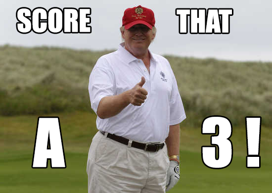
I, myself, made the case for calling him “The Bogey President” which was a reference both to the fact that Trump cheats at golf and Mister Charlie who runs the Bogey Plantation.

But I don’t rank, so it went nowhere.

What to do? Like I said, I’ve put nickname distribution behind me. The above attempt notwithstanding, I have mixed feelings about doing it even to Trump. The only two people who could probably get a nickname to stick to Trump are Vladimir Putin and Xi Jinping. There are no winners when dictators come to blows. When the autocrat’s cage match starts, the whole world loses.

Besides, we are past the point where a nickname for Trump matters. What was Mussolini’s nickname? He was called “Il Duce” (the leader). You may have guessed that it was a nickname he picked for himself. We can imagine some Italian child holding his mother’s hand and asking, “Who is that hanging by his heals from the streetlamp?” The mother looks down at her son and answers: “Il Duce”.