What People Write about Climate: Twitter Data Clustering in Python

Clustering of Twitter data with K-Means, TF-IDF, Word2Vec, and Sentence-BERT

What do people think and write about the climate, pandemics, war, or any other burning issue? Questions like this are interesting from a sociological perspective; knowing the current trends in people’s opinions can also be interesting for scientists, journalists, or politicians. But how can we get answers? Collecting responses from millions of people could have been an expensive process in the past, but today we can get these answers from social network posts. Many social platforms are available nowadays; I selected Twitter for the analysis based on several reasons:

• Twitter was originally designed for making short posts, which could be easier to analyze. At least I hope that while having text size limitations, people try to share their thoughts in a more laconic way.
• Twitter is a large social network; it was founded almost 20 years ago. It has about 450 million active users at the time of writing this article, so it is easy to get plenty of data to work with.
• Twitter has an official API, and its license allows us to use the data for research purposes.

The whole analysis may be pretty complex, and to make the process more clear, let's first describe the steps we need to implement.

Methodology

Our data processing pipeline will consist of several steps.

• Collecting tweets and saving them in a CSV file.
• Cleaning the data.
• Converting the text data into numerical form. I will use 3 methods (TF-IDF, Word2Vec, and Sentence-BERT) to get text embeddings, and we will see which one is better.
• Clustering the numerical data using the K-Means algorithm and analyzing the results. For data visualization, I will use t-SNE (t-distributed Stochastic Neighbor Embedding) methods, and we will also build a word cloud for the most interesting clusters.

Without further ado, let’s get right into it.

1. Loading the data

Collecting the data from Twitter is straightforward. Twitter has an official API and a developer portal; a free account is limited to one project, which is enough for this task. A free account allows us to get recent tweets for only the last 7 days. I collected data within a month, and it was not a problem to run the code once per week. It can be done manually or it can be automated using Apache Airflow, Cron, GitHub Actions, or any other tool. If historical data is really needed, Twitter also has a special academic research access program.

After free registration in the portal, we can get an API “key” and “secret” for our project. For accessing the data, I was using a “tweepy” Python library. This code allows us to get all tweets with a “#climate” hashtag and save them in a CSV file:

import tweepy


api_key = "YjKdgxk..."
api_key_secret = "Qa6ZnPs0vdp4X...."

auth = tweepy.OAuth2AppHandler(api_key, api_key_secret)
api = tweepy.API(auth, wait_on_rate_limit=True)

hashtag = "#climate"

def text_filter(s_data: str) -> str:
    """ Remove extra characters from text """
    return s_data.replace("&", "and").replace(";", " ").replace(",", " ") \
                 .replace('"', " ").replace("\n", " ").replace("  ", " ")

def get_hashtags(tweet) -> str:
    """ Parse retweeted data """
    hash_tags = ""
    if 'hashtags' in tweet.entities:
        hash_tags = ','.join(map(lambda x: x["text"], tweet.entities['hashtags']))
    return hash_tags

def get_csv_header() -> str:
    """ CSV header """
    return "id;created_at;user_name;user_location;user_followers_count;user_friends_count;retweets_count;favorites_count;retweet_orig_id;retweet_orig_user;hash_tags;full_text"

def tweet_to_csv(tweet):
    """ Convert a tweet data to the CSV string """
    if not hasattr(tweet, 'retweeted_status'):
        full_text = text_filter(tweet.full_text)
        hasgtags = get_hashtags(tweet)
        retweet_orig_id = ""
        retweet_orig_user = ""
        favs, retweets = tweet.favorite_count, tweet.retweet_count
    else:
        retweet = tweet.retweeted_status
        retweet_orig_id = retweet.id
        retweet_orig_user = retweet.user.screen_name
        full_text = text_filter(retweet.full_text)
        hasgtags = get_hashtags(retweet)
        favs, retweets = retweet.favorite_count, retweet.retweet_count
    s_out = f"{tweet.id};{tweet.created_at};{tweet.user.screen_name};{addr_filter(tweet.user.location)};{tweet.user.followers_count};{tweet.user.friends_count};{retweets};{favs};{retweet_orig_id};{retweet_orig_user};{hasgtags};{full_text}"
    return s_out


pages = tweepy.Cursor(api.search_tweets, q=hashtag, tweet_mode='extended',
                      result_type="recent",
                      count=100,
                      lang="en").pages(limit)

with open("tweets.csv", "a", encoding="utf-8") as f_log:
    f_log.write(get_csv_header() + "\n")
    for ind, page in enumerate(pages):
        for tweet in page:
            # Get data per tweet
            str_line = tweet_to_csv(tweet)
            # Save to CSV
            f_log.write(str_line + "\n")

As we see, we can get a text body, hashtags, and a user id for each tweet, but if the tweet was retweeted, we need to get the data from the original one. Other fields, like the number of likes, retweets, geo coordinates, etc., are optional but can also be interesting for future analysis. A “wait_on_rate_limit” parameter is important; it allows the library to automatically make a pause if the free limit of API calls is reached.

After running this code, I’ve got about 50,000 tweets with the hashtag “#climate”, posted within the last 7 days.

2. Text Cleaning and Transformation

Cleaning the data is one of the challenges in natural language processing, especially when parsing social network posts. Interestingly, there is no “only right” approach to that. For example, hashtags can contain important information, but sometimes users just copy-paste the same hashtags into all their messages, so the relevance of the hashtags to the message body can vary. Unicode emoji symbols can also be cleaned, but it may be better to convert them into text, and so on. After some experiments, I developed a conversion pipeline, that may not be perfect, but it works well enough for this task.

URLs and Mentioned user names

Many users just post tweets with URLs, often without any comments. It is nice to keep the fact that the URL was posted, so I converted all URLs to the virtual “#url” tag:

import re

output = re.sub(r"https?://\S+", "#url", s_text)  # Replace links with '#url'

Twitter users often mention other people in the text using the “@” tag. User names are not relevant to the text context, and even more, names like “@AngryBeaver2021” are only adding noise to the data, so I removed them all:

output = re.sub(r'@\w+', '', output)  # Remove mentioned user names @... 

Hashtags

Converting hashtags is more challenging. First, I converted the sentence to tokens using NLTK TweetTokenizer:

from nltk.tokenize import TweetTokenizer

s = "This system combines #solar with #wind turbines. #ActOnClimate now. #Capitalism #climate #economics"
tokens = TweetTokenizer().tokenize(s)
print(tokens)
# > ['This', 'system', 'combines', '#solar', 'with', '#wind', 'turbines', '.', '#ActOnClimate', 'now', '.', '#capitalism', '#climate', '#economics']

It works, but it is not enough. People often use hashtags in the middle of the sentence, something like “important #news about the climate”. In that case, the word “news” is important to keep. At the same time, users often add a bunch of hashtags at the end of each message, and in most cases, those hashtags are just copied and pasted and not directly relevant to the text itself. So, I decided to remove hashtags only at the end of the sentence:

while len(tokens) > 0 and tokens[-1].startswith("#"):
    tokens = tokens[:-1]
# Convert array of tokens back to the phrase
s = ' '.join(tokens)

This is better, but it is still not good enough. People often combine several words in one hashtag, like “#ActOnClimate” from the last example. We can split this one into three words:

tag = "#ActOnClimate"
res = re.findall('[A-Z]+[^A-Z]*', tag)
s = ' '.join(res) if len(res) > 0 else tag[1:]
print(s)
# > Act On Climate

As a final result of this step, the phrase “This system combines #solar with #wind turbines. #ActOnClimate now. #Capitalism #climate #economics” will be converted into “This system combines #solar with #wind turbines. Act On Climate now.”.

Removing short tweets

Many users often post pictures or videos without providing any text at all. In that case, the message body is almost empty. These posts are mostly useless for analysis, so I keep in the dataframe only sentences longer than 32 characters.

Lemmatization

Lemmatization is the process of converting words into their original, canonical form.

import spacy
nlp = spacy.load('en_core_web_sm')

s = "I saw two mice today!"

print(" ".join([token.lemma_ for token in nlp(s)]))
# > I see two mouse today !

Lemmatizing the text can reduce the number of words in the text, and the clustering algorithm may work better. A spaCy lemmatizer is analyzing the whole sentence; for example, the phrases “I saw a mouse” and “cut wood with a saw” will provide different results for the word “saw”. Thus, the lemmatizer should be called before cleaning the stopwords.

These steps are enough to clean up tweets. Of course, nothing is perfect, but for our task, it looks good enough. For readers who would like to do experiments on their own, the full code is presented below:

import re
import pandas as pd
from nltk.tokenize import TweetTokenizer

from nltk.corpus import stopwords
stop = set(stopwords.words("english"))

import spacy
nlp = spacy.load('en_core_web_sm')


def remove_stopwords(text) -> str:
    """ Remove stopwords from text """
    filtered_words = [word for word in text.split() if word.lower() not in stop]
    return " ".join(filtered_words)

def expand_hashtag(tag: str):
    """ Convert #HashTag to separated words.
    '#ActOnClimate' => 'Act On Climate'
    '#climate' => 'climate' """
    res = re.findall('[A-Z]+[^A-Z]*', tag)
    return ' '.join(res) if len(res) > 0 else tag[1:]

def expand_hashtags(s: str):
    """ Convert string with hashtags.
    '#ActOnClimate now' => 'Act On Climate now' """
    res = re.findall(r'#\w+', s) 
    s_out = s
    for tag in re.findall(r'#\w+', s):
        s_out = s_out.replace(tag, expand_hashtag(tag))
    return s_out

def remove_last_hashtags(s: str):
    """ Remove all hashtags at the end of the text except #url """
    # "Change in #mind AP #News #Environment" => "Change in #mind AP"
    tokens = TweetTokenizer().tokenize(s)
    # If the URL was added, keep it
    url = "#url" if "#url" in tokens else None
    # Remove hashtags
    while len(tokens) > 0 and tokens[-1].startswith("#"):
        tokens = tokens[:-1]
    # Restore 'url' if it was added
    if url is not None:
        tokens.append(url)
    return ' '.join(tokens) 

def lemmatize(sentence: str) -> str:
    """ Convert all words in sentence to lemmatized form """
    return " ".join([token.lemma_ for token in nlp(sentence)])

def text_clean(s_text: str) -> str:
    """ Text clean """
    try:
        output = re.sub(r"https?://\S+", "#url", s_text)  # Replace hyperlinks with '#url'
        output = re.sub(r'@\w+', '', output)  # Remove mentioned user names @... 
        output = remove_last_hashtags(output)  # Remove hashtags from the end of a string
        output = expand_hashtags(output)  # Expand hashtags to words
        output = re.sub("[^a-zA-Z]+", " ", output) # Filter
        output = re.sub(r"\s+", " ", output)  # Remove multiple spaces
        output = remove_stopwords(output)  # Remove stopwords
        return output.lower().strip()
    except:
        return ""

def text_len(s_text: str) -> int:
    """ Length of the text """
    return len(s_text)


df = pd.read_csv("tweets.csv", sep=';', dtype={'id': object, 'retweet_orig_id': object, 'full_text': str, 'hash_tags': str}, lineterminator='\n')
df['text_clean'] = df['full_text'].map(text_clean)

df['text_len'] = df['text_clean'].map(text_len)
df = df[df['text_len'] > 32]

display(df)

As a bonus, with clean text, we can easily draw a word cloud:

from wordcloud import WordCloud
import matplotlib.pyplot as plt  

def draw_cloud(column: pd.Series, stopwords=None):
    all_words = ' '.join([text for text in column]) 
    
    wordcloud = WordCloud(width=1600, height=1200, random_state=21, max_font_size=110, collocations=False, stopwords=stopwords).generate(all_words) 
    plt.figure(figsize=(16, 12)) 
    plt.imshow(wordcloud, interpolation="bilinear") 
    plt.axis('off')
    plt.show()
    
    
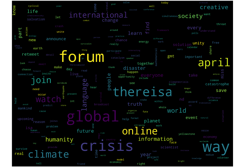
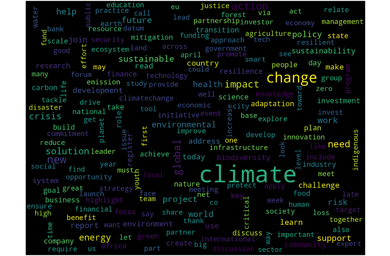
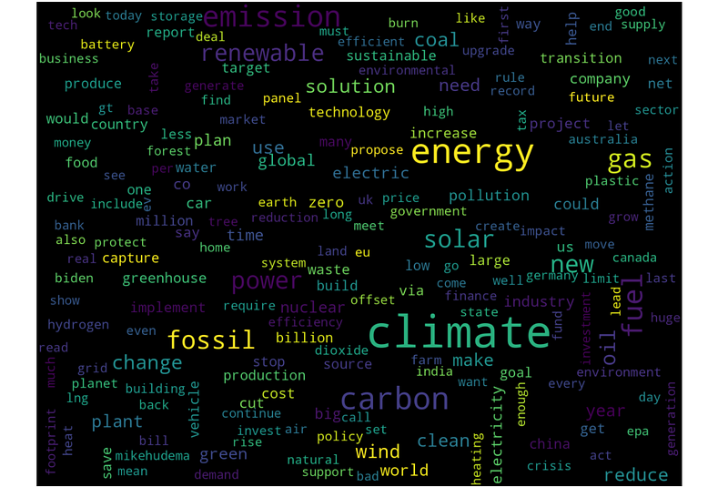
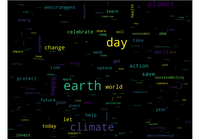
draw_cloud(df['text_clean'])

The result looks like this:

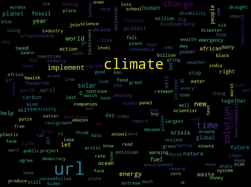
It's not a real analysis yet but this image can already give some insights into what people write about the climate. For example, we can see that often people post links (“URL” is the biggest word in the cloud), and words like “energy”, “waste”, “fossil”, or “crisis” are also relevant and important.

3. Vectorization

Text vectorization is the process of converting text data into a numerical representation. Most of the algorithms, including K-Means clustering as well, require vectors and not plain text. And the conversion itself is not straightforward. The challenge is not just to somehow assign some random vectors to all words; ideally, the words-to-vector conversion should keep the relationship between those words in the original language.

I will test three different approaches, and we can see the advantages and disadvantages of each one.

TF-IDF

TF-IDF (Term Frequency-Inverse Document Frequency) is a pretty old algorithm; a term-weighting function known as IDF was already proposed in the 1970s. The TF-IDF result is based on a numerical statistic, where the TF (term frequency) is the number of times the word appeared in the document (in our case, in the tweet), and the IDF (inverse document frequency) shows how often the same word appears in the text corpus (full set of documents). The higher the score of the particular word, the more important this word is in the specific tweet.

Before processing the real dataset, let’s consider a toy example. Two tweets, cleaned from stop words, the first one is about climate, and the second is about cats:

from sklearn.feature_extraction.text import TfidfVectorizer

docs = ["climate change . information about climate important", 
        "my cat cute . love cat"]

tfidf = TfidfVectorizer()
vectorized_docs = tfidf.fit_transform(docs).todense()

print("Shape:", vectorized_docs.shape)
display(pd.DataFrame(vectorized_docs, columns=tfidf.get_feature_names_out()))

The result looks like this:

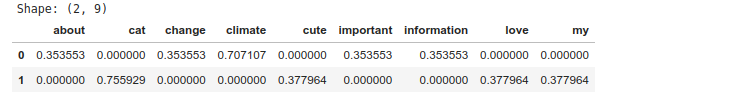
As we can see, we got two vectors from two tweets. Each digit in the vector is proportional to the “importance” of the word in the particular tweet. For example, the word “climate” was repeated twice in the first tweet. It has a high value there and a zero value in the second tweet (and obviously, the output for the word “cat” is the opposite).

Let’s try the same approach on a real dataset we collected before:

docs = df["text_clean"].values

tfidf = TfidfVectorizer()
vectorized_docs = np.asarray(tfidf.fit_transform(docs).todense())

print("Shape:", vectorized_docs.shape)
# > Shape: (19197, 22735)

TfidfVectorizer did the job; it converted each tweet to a vector. The dimension of vectors is equal to the total number of words in the corpus, which is pretty large. In my case, 19,197 tweets have 22,735 unique tokens, and as an output, I got a matrix of the 19,197x22,735 shape! Using such a matrix can be challenging, even for modern computers.

We will cluster this data in the next step, but before that, let's test other vectorization methods.

Word2Vec

Word2Vec is another approach for word vectorization; the first paper about this method was introduced by Tomas Mikolov in 2013 at Google. There are different algorithms (Skip-gram and CBOW models) available in the implementation; the general idea is to train the model on a large text corpus and get accurate word-to-vector representations. This model is able to learn the relations between different words, as shown in the original paper:

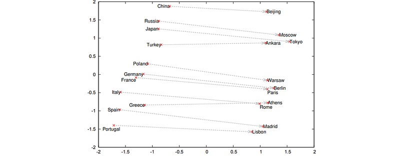
Probably the most famous example of using this model is the relationship between the words “king”, “man” and “queen”. Those who are interested in details can read this nice article.

For our task, I will be using a pre-trained vector file. This model was trained using the Google News dataset; the file contains vectors for 3 million words and phrases. Before using a real dataset, let’s again consider a toy example:

from gensim.models import Word2Vec, KeyedVectors
from gensim.models.doc2vec import Doc2Vec, TaggedDocument


word_vectors = KeyedVectors.load_word2vec_format('GoogleNews-vectors-negative300.bin', binary=True)

print("Shape:", word_vectors["climate"].shape)
display(word_vectors["climate"])

The result looks like this:

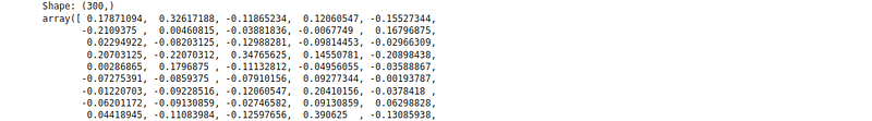
As we can see, the word “climate” was converted into a 300-digit length array.

Using Word2Vec, we can get embeddings for each word, but we need an embedding for the whole tweet. As the easiest approach, we can use the word embedding arithmetic and get the mean of all vectors:

from nltk import word_tokenize


def word2vec_vectorize(text: str):
    """ Convert text document to the embedding vector """    
    vectors = []
    tokens = word_tokenize(text)
    for token in tokens:
        if token in word_vectors:
            vectors.append(word_vectors[token])
            
    return np.asarray(vectors).mean(axis=0) if len(vectors) > 0 else np.zeros(word_vectors.vector_size)

This works because words with similar meanings are converted into close vectors, and vice versa. With this method, we can convert all our tweets into embedding vectors:

docs = df["text_clean"].values

vectorized_docs = list(map(word2vec_vectorize, docs))
print("Shape:", vectorized_docs.shape)

# > Shape: (22535, 300)

As we can see, Word2Vec’s output is much more memory-efficient compared to the TF-IDF approach. We have 300-dimensional vectors for each tweet, and the shape of the output matrix is 19,197x300 instead of 19,197x22,735 — a 75x difference in memory footprint!

Doc2Vec is another model that can be more effective for making document embeddings compared to “naive” averaging; it was specially designed for vector representations of the documents. But at the time of writing this article, I was not able to find a pre-trained Doc2Vec model. Readers are welcome to try this on their own.

Sentence-BERT

In the previous step, we got word embeddings using Word2Vec. It works, but this approach has an obvious disadvantage. Word2Vec does not respect the context of the word; for example, the word “bank” in the sentence “the river bank” will get the same embedding as “the bank of England”. To fix that and get more accurate embeddings, we can try a different approach. The BERT (Bidirectional Encoder Representations from Transformer) language model was introduced in 2018. It was trained on masked text sentences, in which the position and context of each word really matter. BERT was not originally made for calculating embeddings, but it turned out that extracting embeddings from BERT layers is an effective approach (those TDS articles from 2019 and 2020 can provide more details: 1, 2).

Nowadays, several years later, the situation has improved, and we don’t need to extract raw embeddings from BERT manually; special projects like Sentence Transformers were specially designed for that. Before processing a real dataset, let’s consider a toy example:

from sentence_transformers import SentenceTransformer


docs = ['the influence of human activity on the warming of the climate system has evolved from theory to established fact', 
        'cats can jump 5 times their own height']

model = SentenceTransformer('all-MiniLM-L6-v2')
vectorized_docs = model.encode(np.asarray(docs))

print("Shape:", vectorized_docs.shape)
# > Shape: (2, 384)

As an output, we got two 384-dimensional vectors for our sentences. As we can see, using the model is easy, and even removing the stop words is not required; the library is doing all this automatically.

Let’s now get embeddings for our tweets. Since BERT word embeddings are sensitive to word context and the library has its own cleaning and tokenization, I will not use the “text_clean” column as before. Instead, I will only convert tweet URLs and hashtags to text. The “partial_clean” method uses parts of the code from the original “text_clean” function, used at the beginning of this article:

def partial_clean(s_text: str) -> str:
    """ Convert tweet to a plain text sentence """
    output = re.sub(r"https?://\S+", "#url", s_text)  # Replace hyperlinks with '#url'
    output = re.sub(r'@\w+', '', output)  # Remove mentioned user names @... 
    output = remove_last_hashtags(output)  # Remove hashtags from the end of a string
    output = expand_hashtags(output)  # Expand hashtags to words
    output = re.sub(r"\s+", " ", output)  # Remove multiple spaces
    return output


docs = df['full_text'].map(partial_clean).values
vectorized_docs = model.encode(np.asarray(docs))
print("Shape:", vectorized_docs.shape)

# > Shape: (19197, 384)

As an output of the sentence transformer, we got an array of 19,197x384 dimensionality.

As a side note, it is important to mention that the BERT model is much more computationally “heavy” compared to Word2Vec. Calculating vectors for 19,197 tweets took about 80 seconds on a 12-core CPU, compared to only 1,8 seconds required by Word2Vec. It is not a problem for doing tests like this, but it can be more expensive to use in a cloud environment.

4. Clustering and Visualization

Finally, we’re approaching the last part of this article. During previous steps, we got 3 versions of the “vectorized_docs” array, generated by using 3 methods: TF-IDF, Word2Vec, and Sentence-BERT. Let’s cluster these embeddings into groups and see what information we can extract.

To do this, let’s first make several helper functions:

from sklearn.cluster import KMeans
from sklearn.metrics import silhouette_score


def make_clustered_dataframe(x: np.array, k: int) -> pd.DataFrame:
    """ Create a new dataframe with original docs and assigned clusters """
    ids = df["id"].values
    user_names = df["user_name"].values
    docs = df["text_clean"].values
    tokenized_docs = df["text_clean"].map(text_to_tokens).values
    
    km = KMeans(n_clusters=k).fit(x)
    s_score = silhouette_score(x, km.labels_)
    print(f"K={k}: Silhouette coefficient {s_score:0.2f}, inertia:{km.inertia_}")
    
    # Create new DataFrame
    data_len = x.shape[0]
    df_clusters = pd.DataFrame({
        "id": ids[:data_len],
        "user": user_names[:data_len],
        "text": docs[:data_len],
        "tokens": tokenized_docs[:data_len],
        "cluster": km.labels_,
    })
    return df_clusters


def text_to_tokens(text: str) -> List[str]:
    """ Generate tokens from the sentence """
    # "this is text" => ['this', 'is' 'text']
    tokens = word_tokenize(text)  # Get tokens from text
    tokens = [t for t in tokens if len(t) > 1]  # Remove short tokens
    return tokens


# Make clustered dataframe
k = 30
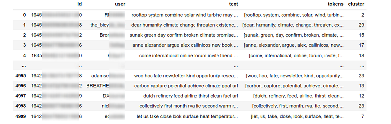
df_clusters = make_clustered_dataframe(vectorized_docs, k)
with pd.option_context('display.max_colwidth', None):
    display(df_clusters)

I am using SciKit-learn KMeans to make K-Means clustering. A “make_clustered_dataframe” method creates a dataframe with original tweets and a new “cluster” column. When using K-Means, we also have two metrics that help us evaluate the results. Inertia can be used to measure clustering quality. It is calculated by measuring the distance between all cluster points and cluster centroids, and the lower the value, the better. Another useful metric is the silhouette score; this value has a range of [-1, 1]. If the value is close to 1, the clusters are well separated; if the value is about 0, the distance is not significant; and if the values are negative, the clusters are overlapping.

The output of “make_clustered_dataframe” looks like this:

It works, but only using this information, it’s hard to see if the clusters are good enough. Let’s add another helper method to display the top clusters, sorted by silhouette score. I use the SciKit-learn silhouette_samples method to calculate this. I will also use a word cloud to visualize each cluster:

from sklearn.metrics import silhouette_samples


def show_clusters_info(x: np.array, k: int, cdf: pd.DataFrame):
    """ Print clusters info and top clusters """
    labels = cdf["cluster"].values
    sample_silhouette_values = silhouette_samples(x, labels)
    
    # Get silhouette values per cluster    
    silhouette_values = []
    for i in range(k):
        cluster_values = sample_silhouette_values[labels == i]
        silhouette_values.append((i, 
                                  cluster_values.shape[0], 
                                  cluster_values.mean(), 
                                  cluster_values.min(), 
                                  cluster_values.max()))
    # Sort
    silhouette_values = sorted(silhouette_values, 
                               key=lambda tup: tup[2], 
                               reverse=True)
    
    # Show clusters, sorted by silhouette values
    for s in silhouette_values:
        print(f"Cluster {s[0]}: Size:{s[1]}, avg:{s[2]:.2f}, min:{s[3]:.2f}, max: {s[4]:.2f}")

    # Show top 7 clusters
    top_clusters = []
    for cl in silhouette_values[:7]:
        df_c = cdf[cdf['cluster'] == cl[0]]

        # Show cluster
        with pd.option_context('display.max_colwidth', None):
            display(df_c[["id", "user", "text", "cluster"]])
            
        # Show words cloud
        s_all = ""
        for tokens_list in df_c['tokens'].values:
            s_all += ' '.join([text for text in tokens_list]) + " "            
        draw_cloud_from_words(s_all, stopwords=["url"])
        
        # Show most popular words
        vocab = Counter()
        for token in df_c["tokens"].values:
            vocab.update(token)
        display(vocab.most_common(10))


def draw_cloud_from_words(all_words: str, stopwords=None):
    """ Show the word cloud from the list of words """
    wordcloud = WordCloud(width=1600, height=1200, random_state=21, max_font_size=110, collocations=False, stopwords=stopwords).generate(all_words) 
    plt.figure(figsize=(16, 12)) 
    plt.imshow(wordcloud, interpolation="bilinear") 
    plt.axis('off')
    plt.show()


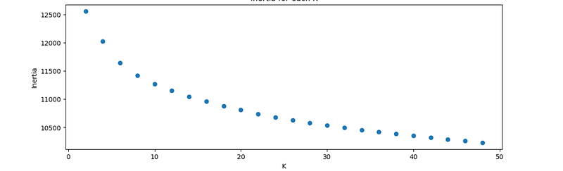
show_clusters_info(vectorized_docs, k, df_clusters)

The next important question before using the K-Means method is choosing the “K”, optimal number of clusters. The Elbow method is a popular technique; the idea is to build the inertia value graph for different K-values. The “elbow” point on the graph is (at least in theory) the value of optimum K. Practically, it rarely works as expected, especially for badly structured datasets such as vectorized tweets, but the graph can give some insights. Let’s make a helper method to draw the elbow graph:

import matplotlib.pyplot as plt  
%matplotlib inline


def graw_elbow_graph(x: np.array, k1: int, k2: int, k3: int):
    k_values, inertia_values = [], []
    for k in range(k1, k2, k3):
        print("Processing:", k)
        km = KMeans(n_clusters=k).fit(x)
        k_values.append(k)
        inertia_values.append(km.inertia_)

    plt.figure(figsize=(12,4))
    plt.plot(k_values, inertia_values, 'o')
    plt.title('Inertia for each K')
    plt.xlabel('K')
    plt.ylabel('Inertia')


graw_elbow_graph(vectorized_docs, 2, 50, 2)

Visualization

As a bonus point, let’s add the last (I promise, it’s the last:) helper method to draw all clusters on a 2D plane. I suppose most readers cannot visualize 300-dimensional vectors in their heads yet ;) so I will use t-SNE (T-distributed Stochastic Neighbor Embedding) dimensionality reduction methods to reduce the number of dimensions to 2, and Bokeh to draw the results:

from sklearn.decomposition import PCA
from sklearn.manifold import TSNE

from bokeh.io import show, output_notebook, export_png
from bokeh.plotting import figure, output_file
from bokeh.models import ColumnDataSource, LabelSet, Label, Whisker, FactorRange
from bokeh.transform import factor_cmap, factor_mark, cumsum
from bokeh.palettes import *
from bokeh.layouts import row, column
output_notebook()


def draw_clusters_tsne(docs: List, cdf: pd.DataFrame):
    """ Draw clusters using TSNE """
    cluster_labels = cdf["cluster"].values
    cluster_names = [str(c) for c in cluster_labels]
    
    tsne = TSNE(n_components=2, verbose=1, perplexity=50, n_iter=300, 
                init='pca', learning_rate='auto')
    tsne_results = tsne.fit_transform(vectorized_docs)

    # Plot output
    x, y = tsne_results[:, 0], tsne_results[:, 1]
    source = ColumnDataSource(dict(x=x, 
                                   y=y, 
                                   labels=cluster_labels,
                                   colors=cluster_names))
    palette = (RdYlBu11 + BrBG11 + Viridis11 + Plasma11 + Cividis11 + RdGy11)[:len(cluster_names)]

    p = figure(width=1600, height=900, title="")
    p.scatter("x", "y",
              source=source, fill_alpha=0.8, size=4,
              legend_group='labels',
              color=factor_cmap('colors', palette, cluster_names)
              )
    show(p)
    

draw_clusters_tsne(vectorized_docs, df_clusters)

Now that we are ready to see the results, let’s see what we can get.

Results

I was using three different (TF-IDF, Word2Vec, and Sentence-BERT) algorithms to convert text into embedding vectors, which are seriously different in architecture. Will all of them be able to find interesting patterns in all tweets? Let’s examine the results.

TF-IDF

The major disadvantage of finding clusters in TF-IDF embeddings is a large amount of data. In my case, the matrix size was 19,197x22,735, because the text corpus contains 19,197 tweets and 22,735 unique tokens. Finding clusters in a matrix of that size is not fast, even for a modern PC.

In general, TF-IDF vectorization did not provide exceptional results, but K-Means was still able to find some interesting clusters. For example, from all 19,197 tweets, a 200-tweet cluster was detected in which people were making posts about the international online forum:

K-Means was also able to find some users who made a lot of similar posts:

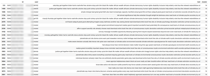
In this case, a user with the nickname “**mickel” was probably trying to promote his online book (by the way, showing the message ids is useful for debugging; we can always open the original tweet in the browser), and he published a lot of similar posts about that. Those posts were not absolutely similar, but the algorithm was able to cluster them together. This approach can be useful, for example, in detecting accounts used for posting spam.

Some interesting clusters were found in TF-IDF vectors, but most other clusters had silhouette values around zero. The t-SNE visualization shows the same result. There are some local groups in the picture, but most of the points overlap each other:

I saw some articles where authors got good results with TF-IDF embeddings, mostly in cases where texts belong to different domains. For example, posts about “politics”, “sports,” and “religion” will likely form more isolated clusters with higher silhouette values. But in our case, all texts are about climate, so the task is more challenging.

Word2Vec

The first interesting result with Word2Vec — the Elbow method was able to produce a somehow visible “elbow” point:

With K=8, the t-SNE visualization gave this result:

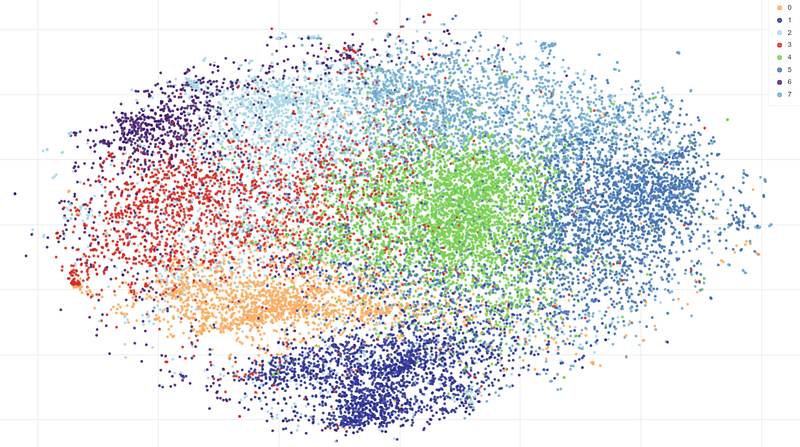
Most of the clusters are still overlapping, and silhouette values are, in general, low. But some interesting patterns can be found.

“Climate change”. This cluster has the most popular words “climate”, “change”, “action,” and “global”:

Lots of people are obviously worried about climate change, so having this cluster is obvious.

“Fuels”. This cluster has popular words like “energy”, “carbon”, “emission”, “fossil,” or “solar”:

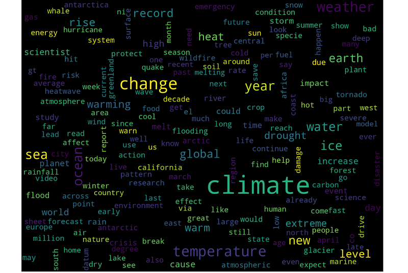
“Environment”. Here we can see such words as “temperature”, “ocean”, “sea”, “ice,” and so on.

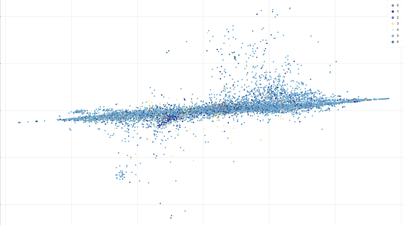
Sentence-BERT

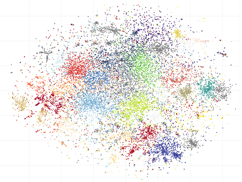
In theory, these embeddings should provide the most accurate results; let’s see how it is going. A t-SNE cluster visualization looks like this:

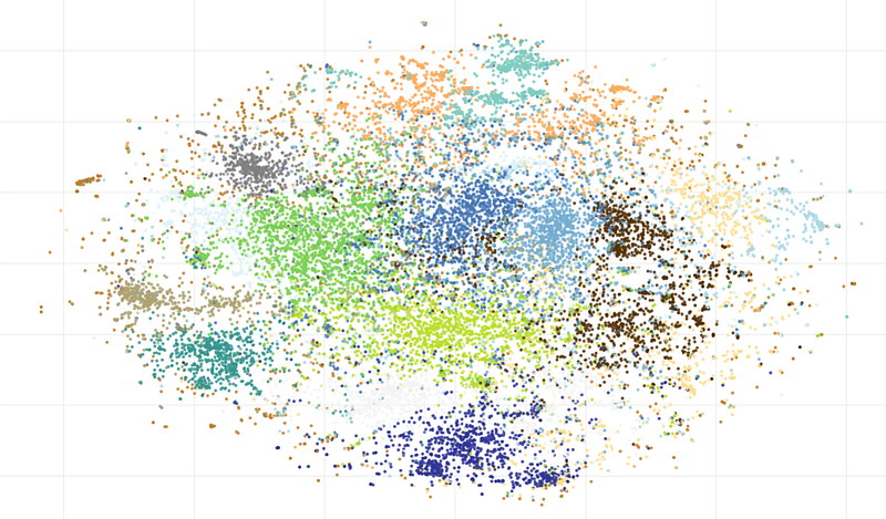
As we can see, many local clusters can be found, and I will show some of the most interesting of them.

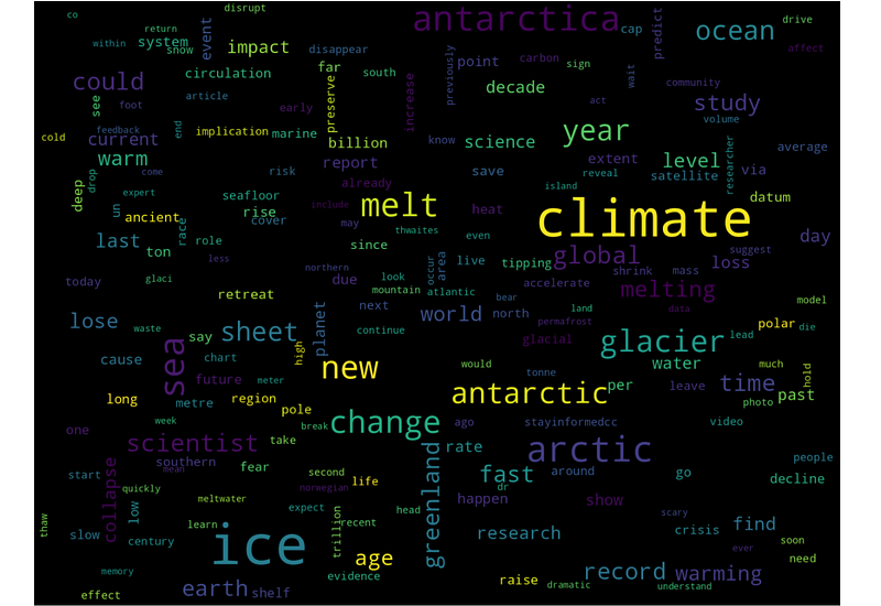
“Ice melting”. A cluster with the most popular words “climate”, “ice”, “melt”, “glacier”, and “arctic”:

“Earth day”. This day is celebrated in April when this data was collected, and there is a cluster of messages with words like “earth”, “day”, “planet”, “happy”, or “action”:

“Global international forum”:

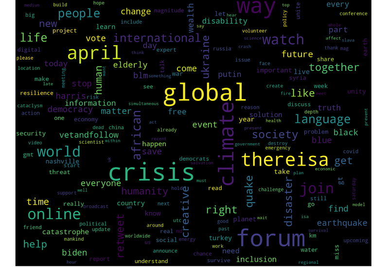
This result is interesting for two reasons. Firstly, we saw this cluster before; the K-Means algorithm found it in the TF-IDF embeddings. Secondly, the “Word2Vec” model did not have the word “thereisa” in the dictionary, so it was just skipped. BERT has a better tokenization scheme, in which the unknown words are split into smaller tokens. We can easily see how it works:

model = SentenceTransformer('all-MiniLM-L6-v2')

inputs = model.tokenizer(["thereisa online forum"])
tokens = [e.tokens for e in inputs.encodings]

print(tokens)
# > [['[CLS]', 'there', '##isa', 'online', 'forum', '[SEP]']]

We can see that the words “online” and “forum” were converted into single tokens, but the word “thereisa” was converted into two words “there” and “##isa”. This not only allows BERT to deal with unknown words, but it is actually much closer to what we, as humans, often do: when we see unknown words, we often try to “split” them into pieces and guess the meaning.

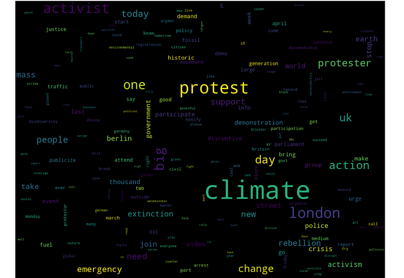
But let’s go further. Another distinct group is related to protests; we can see here such words as “protest, “change”, “action”, “activism“, and so on:

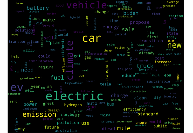
And last but not least, another popular climate-related topic is electric transport. Here we can see words like “new”, “electric”, “car”, or “emission”:

Conclusion

Using text clustering, we were able to process raw and unstructured text from social networks (in our case, Twitter, but this approach should also work with other platforms) and find interesting and distinctive patterns in the posts of tens of thousands of users. This can be important not only for purely academic reasons like cultural anthropology or sociology studies but also for “pragmatic” cases like detecting bots or users posting spam.

From a natural language processing perspective, clustering social media data is an interesting and challenging topic. It is challenging because there are many ways of cleaning and transforming the data, and no way would be perfect. In our case, BERT embeddings unsurprisingly provided the best results compared to earlier TF-IDF and Word2Vec models. BERT is not only giving good results, but it is also better for dealing with unknown words, which can be a problem with Word2Vec. TF-IDF embeddings, in my opinion, did not show any exceptional results, but this approach still has an advantage. TF-IDF is based on pure statistics, and it does not require a pre-trained language model. So, in the case of rare languages for which pre-trained models are not available, TF-IDF can be used.

This article provides a sort of “low-level” approach, which is better for understanding how things work, and I encourage readers to do some experiments on their own; the source code in the article should be enough for that. At the same time, those who just want to get results in 10 lines of code without thinking about what is “under the hood”, are welcome to try ready-to-use libraries like BERTopic.

If you enjoyed this story, feel free to subscribe to Medium, and you will get notifications when my new articles will be published, as well as full access to thousands of stories from other authors.

Thanks for reading.