
What is the Curse of Dimensionality?
The curse of dimensionality refers to various problems that arise when working with high-dimensional data. In this article we will discuss these problems and how they affect machine learning algorithms, and then suggest a few ways to deal with them.
Living in a High-Dimensional Space
We are so used to live in three dimensions, that our intuition fails when we try to imagine things in high-dimensional spaces. Many things behave very differently in high-dimensional spaces.
For example, if we pick a random point in a unit square (a square whose side length is 1), its probability of being located less than 0.01 from the border of the square is less than 2%. This is because the area of the unit square is 1, whereas the area of the inner square with side length 0.99 is 0.99 × 0.99 = 0.9801. Therefore, the probability that the point falls inside the area between the inner square and the unit square is 1–0.9801 = 0.0199.
On the other hand, if we pick a random point in a unit hypercube with 1,000 dimensions, its probability of being located less than 0.01 from the border of the hypercube is greater than 99.99%!
The reason is that the volume of the unit hypercube is 1¹⁰⁰⁰ = 1, while the volume of the inner hypercube with side length of 0.99 is 0.99¹⁰⁰⁰ = 0.00004317. Therefore, the probability that the point falls inside the volume between the inner hypercube and the unit hypercube is 1–0.00004317 = 0.99995683.
This means that high-dimensional spaces are very sparse, i.e., most of the data points lie very close to the border of the surface, and thus are very far from each other.
Nearest Neighbor Search
This effect complicates nearest neighbor search in high-dimensional spaces, since the nearest neighbors in these spaces are not very near!
Consider k-nearest neighbors in a data set of n points that are uniformly distributed inside a d-dimensional unit hypercube. Let the k-neighborhood of a point be the smallest hypercube that contains its k-nearest neighbors, and let l be the average side length of such a neighborhood. Then the volume of the neighborhood (that contains k points) is lᵈ, while the volume of the unit hypercube (that contains n points) is 1. Therefore, on average lᵈ = k/n, or:

In other words, the average side length of a k-neighborhood increases exponentially as the number of dimensions grows (note that the number in the brackets is smaller than 1).
The following graph shows the length of the average neighborhood for 10-nearest neighbors in a unit hypercube with 1,000,000 points, as a function of the number of dimensions:
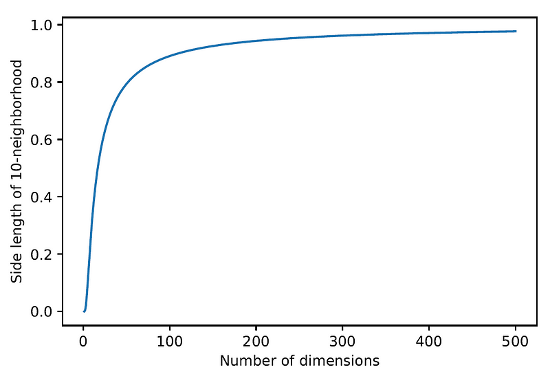
In three dimensions, the average neighborhood has l = 0.021 (only a small fraction of the unit cube), while in 500 dimensions, it is 97.7%!
Similarly, when a distance measure such as Euclidean distance is used in a high-dimensional space, there is little difference in the distances between different pairs of points. This is because the ratio between the nearest and farthest points approaches 1, i.e., the points essentially become uniformly distant from each other.
How does it Affect Machine Learning?
Machine learning algorithms that are based on nearest neighbor search (such as KNN) or on distance measures (such as K-means) suffer from the curse of dimensionality due to the effects mentioned above.
Moreover, as the number of dimensions increases, the amount of data we need to generalize accurately grows exponentially. With a fixed number of training samples, the predictive power of the model first increases as the number of features (dimensions) goes up, but beyond a certain of number of features it starts to deteriorate.
Other issues related to high-dimensionality data are:
- Training the model takes more time.
- The data requires more storage space.
- Interpretation and visualization become much harder in high-dimensional spaces.
Solution: Dimensionality Reduction
In order to deal with the curse of dimensionality, we need to reduce the number of dimensions. There are two main methods to do so:
- Feature selection, i.e., select only a subset of the original features to build the model. Feature selection methods are less effective in data sets with a large number of features (such as images).
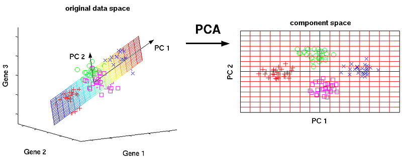
- Use a dimensionality reduction technique such as Principal Component Analysis (PCA). PCA projects the data into a lower-dimensional space that captures the largest amount of variation in the data (i.e., preserves as much information as possible).
Algorithms for feature selection and dimensionality reduction will be covered in more depth in future articles.
Curse of Dimensionality Example
To demonstrate the curse of dimensionality, we will run a K-nearest neighbor search to classify 1,000 random images from the MNIST data set. This data set contains 70,000 images of handwritten digits, and the goal is to classify these images into one of the ten digits (0–9). Each image is 28 × 28 pixels in size, i.e., the number of dimensions is 784.
We will first use all the features (pixels in this case), and then we will see whether we can improve the results by reducing the number of dimensions.
Let’s first fetch the data set using the fetch_openml() function:
from sklearn.datasets import fetch_openml

X, y = fetch_openml('mnist_784', return_X_y=True, as_frame=False)
We now scale the inputs to be within the range [0, 1] instead of [0, 255]:
X = X / 255Let’s pick a random subset of 1,000 samples from the data set:
random_subset = np.random.choice(range(len(X)), size=1000)
X_sample = X[random_subset]
y_sample = y[random_subset]
We now split these samples into 80% training and 20% test:
from sklearn.model_selection import train_test_split

X_train, X_test, y_train, y_test = train_test_split(X_sample, y_sample, test_size=0.2, random_state=0)
Next, we create a KNeighborsClassifier with its default settings (n_neighbors = 5) and fit it to the training set:
from sklearn.neighbors import KNeighborsClassifier

knn = KNeighborsClassifier()
knn.fit(X_train, y_train)
Let’s check the accuracy of the model on the training and the test sets:
print('Accuracy on training set:', knn.score(X_train, y_train))
print('Accuracy on test set:', knn.score(X_test, y_test))
Accuracy on training set: 0.92125
Accuracy on test set: 0.855We get 85.5% accuracy on the test set.
Let’s now use PCA from Scikit-Learn to reduce the number of dimensions from 784 down to 50. To specify the number of dimensions you want to keep, use the parameter n_components in the class constructor:
from sklearn.decomposition import PCA

pca = PCA(n_components=50)
We now call fit_transform() on the training set to reduce the number of dimensions. For the test set, we only need to call transform()
X_train_reduced = pca.fit_transform(X_train)
X_test_reduced = pca.transform(X_test)
Next, we fit the KNeighborsClassifier on the reduced training set:
knn.fit(X_train_reduced, y_train)
The accuracy of the model this time is:
print('Accuracy on training set:', knn.score(X_train_reduced, y_train))
print('Accuracy on test set:', knn.score(X_test_reduced, y_test))
Accuracy on training set: 0.93375
Accuracy on test set: 0.88The accuracy on the test has improved significantly! (from 85.5% to 88%).
Lastly, let’s examine how the accuracy on the test changes as a function of the number of dimensions. To that end, we will reduce the data set to various numbers of dimensions in the range [10, 700] with intervals of 10, and then plot the test accuracy for each number:
dimensions = range(10, 701, 10)
scores = []

for n_dimensions in dimensions:
    pca = PCA(n_components=n_dimensions)
    X_train_reduced = pca.fit_transform(X_train)
    X_test_reduced = pca.transform(X_test)
    knn.fit(X_train_reduced, y_train)
    score = knn.score(X_test_reduced, y_test)
    scores.append(score)
plt.plot(dimensions, scores)
plt.xlabel('Dimensions')
plt.ylabel('Test accuracy')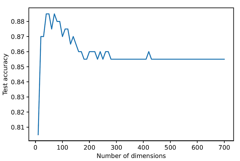
As can be seen, we get the highest accuracy when the number of dimensions is around 50, and then the accuracy consistently drops as we increase the number of dimensions.
Final Notes
The code examples of this article can be found on my github: https://github.com/roiyeho/medium/tree/main/curse_of_dimensionality
Thanks for reading!


